Программное обеспечение прототипа распределенной бортовой вычислительной системы
|
|
|
Introduction |
4 |
|
1. |
Operation
system choice |
5 |
|
1.1. |
Analysis of on-board computer complex software
requirements and OS choice |
5 |
|
1.2. |
Challengers
for on-board OS |
6 |
|
1.3. |
Preliminary
conclusion |
9 |
|
2. |
Determination
of requirements to software for the on-board computer system prototype |
9 |
|
2.1. |
Local module software requirements |
9 |
|
2.2. |
Software
requirements for entire computer complex |
10 |
|
3. |
Development of applied
programs for on-board data processing at the airborne computer system
prototype |
10 |
|
3.1. |
Statement of problem |
11 |
|
3.2. |
Task of
hyper-spectral measurements |
11 |
|
3.3. |
Hyper-spectral
data processing techniques |
12 |
|
3.3.1. |
Correlation
method for experimental data processing |
12 |
|
3.3.2. |
Sub-pixel method for
experimental data processing |
13 |
|
3.4. |
Processing algorithms |
14 |
|
4. |
Algorithms
of initial configuring, routing, and reconfiguring |
19 |
|
4.1. |
System composition |
19 |
|
4.2. |
Initiation stage |
20 |
|
4.3. |
Operation mode |
21 |
|
4.4. |
A module failure |
22 |
|
4.5. |
Types of output data |
22 |
|
4.6. |
Output data compression |
23 |
|
|
References |
24 |
Introduction
The Keldysh
Institute of Applied Mathematics of RAS and the Space Research Institute of RAS
both jointly with the Fraunhofer
Institute Rechnerarchitektur und Softwaretechnik (FIRST, Berlin, Germany) develop
software and instrumental parts for the prototype of an onboard computer system
resistant to some separate failures in a framework of the project № 2323 entitled «The Development of
the Prototype of Distributed Fault Tolerant On-Board Computing System for
Satellite Control System and the Complex of Scientific Equipment» under support
of the International Scientific and Technical Center. This work includes a
development of a fail-safe distributed onboard computer system prototype to
control a spacecraft and the scientific equipment facility making the
hyper-spectral remote sensing of the Earth.
Requirements
to the board and scientific equipment control facility necessary to carry out
the mission’s scientific tasks can be only fulfilled by a powerful and flexible
computer & communication infrastructure. Broad operational variety demands
that the computing functions and capabilities must be adaptable to changing
in-time requirements. The scientific equipment control system closely interacts
with the on board control facility in terms of requirements per concrete
operation. While the on board control complex should provide for a high rate of
the spacecraft’s autonomous operation as well as its robustness as the top
priority task.
The on-Board
Computer System (BCS) is a distributed multi-computer system resistant to
separate failures and accomplishing entire steering, telemetry and monitoring
functions as well as all application functions typical for scientific equipment
and computer control system facility.
Amalgamation of
different computing functions on a spacecraft board into a single system with a
high redundancy rate allows both tight interworking between various processes
and optimizes flexible utilization of the reserved computer resources to
execute different tasks depending on the operation requirements and the
necessary failure resistance level. The on-board computer architecture corresponds
to a homogeneous symmetrical multi-computer system i.e. it comprises several
(from 3 to 16) similar nodal computers linked by a redundant bus system.
Actually each computer is able to execute any process and has an access to
every I/O-channel. The software architecture
build-up uses the same approach as the instrumental part architecture. It must
be modular, distributed and reiteratively redundant. The compact kernel
operation system (OS) should provide each node for basic functioning in the
multi-task mode with priorities, the priority based and real time based
planning, communications and memory resources control.
The preprint discusses and substantiates the real time OS choice and
describes the developed application software for the hyper-spectral imaging.
1.
OS choice
1.1.
Analysis of on-board computer complex software requirements and OS choice
It is
understood that the proper computer system architecture choice is only possible
when taking it as a one whole entity combining instrumental and software parts.
The key issue in designing of the instrumental part is the choice of an OS, its kernel and specialized
software (SSW), since the build-up of the whole computer system needs to take
into account which tasks are solved by a hardware and which by a software,
while the work is restricted in time and funding.
Therefore,
at the first stage our attention was drawn to the choice of an OS for on-board
computer system prototype. Let us discuss guiding requirements for the OS choice.
The requirements below are given in the importance descending order.
Satisfaction to the beginning requirement points is the guiding principle for
selection of the concrete OS.
The target
system is understood as a whole computer complex devised to host the OS and
SSW. The computer complex main tasks are seen as tasks carried out by SSW.
1. Functionality requirements:
a)
OS level support for the following issues:
--synchronized objects: spinlocks,
mutexes;
--signals;
--interruptions;
--clocks, timers;
--exceptional cases;
--message queues;
--tasks (processes) with priorities;
--inner task flows (threads) with
priorities;
--memory scheduler;
--external devices;
--shared memory;
--multiprocessor computer systems.
b)
Principal implementation capability to support instrumental interfaces of the
target system within the chosen OS frameworks.
c)
The OS overall usage of the CPU resources, external and internal memory is
rather enough to allow solution of the computer complex main tasks within the
taken OS (~10-100 Kb).
d)
The maximum response delay time to an external instrumental interrupt is within
limits for the lossless data exchange control over any bus provided the CPU
resources consumption leaving rather enough time for the computer complex main
tasks within the taken OS (~1-2 μs).
e) The maximum task relay time is within limits
sufficient for the SSW operation (~1 ms).
f)
The flow relay time inside one task frameworks is within limits sufficient for
the SSW operation (~100 ns).
2. Control and reliability requirements:
а) Availability
of the entire OS source code written in a high level language with clear-cut
structure.
b) The taken
OS must have cross-compiling and cross-debugging tools for at least one common
used OS such as UNIX or Windows.
3. Flexibility and scalability requirements:
a) Presence
of a configuration mechanism (or its development means) as well as OS
installation and loading mechanism for the target system.
b) Presence
of a mechanism (or its development means) to apply the newly developed modules
and components (i.e. drivers for new equipment) in the OS frameworks.
4.Miscellaneous requirements:
a) The taken
OS is desirable to have auxiliary tools facilitating the developers’ work such
as debugger, profiler, utilities for log analysis and acquisition of various
information, etc.
1.2.
Challengers for on-board OS
Hereinafter
+: means advantage
-: means drawback
The following OS were analyzed:
1. eCOS
(http://sources.redhat.com/ecos/)
+: Open
source code system is widely supported by the largest Linux (RedHat) based solution
supplier with implementation (in C++, assembler) for PowerPC (IBM, Xilinx,
Motorola) and many other platforms (the list is being permanently expanded).
The system is compatible with the standard cross-tools of GNU.
-: strict
lock-on to GCC compiler (to a set of compilers to be exact) supplied with GNU
license; the use of other compilers is hardly whatever possible.
2. BOSS
+: Open source code system with quite simple and explicit implementation (in C++, assembler) for PowerPC.
The
OS is compatible with the standard cross-tools of GNU and was previously used
in a satellite computer complex with manifold redundancy. The system showed stable performance for harsh conditions.
-: very
narrow circle of developers; lack of standard equipment support, the OS has no
support for such regnant concepts as kernel modules or network sockets.
3. VxWorks (WindRiver)
+: The
leader of the embedded systems market, the OS was tested in multiple
applications, it is proved to be a high-speed one with a configurable kernel
and the broadest support of different equipment provided with flexible license
(discount for massive purchases). Cross-tools use freely distributed GNU
program packages and company’s own developed utilities for popular OS’s based
on Windows NT and Linux clones are available for developers. There is also a
graphic subsystem optimized for the embedded applications available for
additional charge.
-: The OS
cost is pretty high as compared with the counterparts. The source code is
licensed by the supplier and is provided for considerable extra charge with no
alterations allowed (languages С/C++, assembler). The shared memory system is either
available only for additional charges.
4. Windows NT
hard real-time extensions
+: Windows
NT kernel based systems are able to execute the majority of programs developed
for Windows platform i.e. the target computer may simultaneously be the
developer’s computer.
-: Yet
actually this type system falls into two parts:
the first one works under the old, not real-time kernel control with its
own drivers,
the second one works under the new real-time kernel control rewritten by
manufacturer as a specific solution (a note for specialists: here the NT kernel
is considered as either the "ntoskrnl.exe” itself or tightly linked to it
"hal.dll” and some few similar libraries).
Achilles's heel of this approach is the fact that inside the
non-real-time interrupt controller the interrupts are banned (poor quality
drivers sometimes even themselves do this “for reliability sake”) what
extinguishes any performance speed guaranties for other components. High cost
and at the same time complete source code secrecy of the solution should also
be pointed out. Therefore, even the, so called, “real-time extensions” for the
satellite on-board computer applications do not fully match the reliability
criterion in either cases of at least one standard driver usage or a necessity
to somewhat alter the system response to external events (this is specific for
all closed source code systems).
5. Windows CE
+: The initially
oriented for the mobile computer market is small in size, has fairly good rate
and relatively low cost.
-: Closed
kernel, rather big interrupt response delays, considerably abridged
functionality as compared with Windows NT.
6. Linux real-time extensions
+: such type
systems are the general purpose OS remake substantially slimmed-down (the
kernel had been altered and has open source code), supplemented but rather
remained principally intact. Thus, the majority of already made OS Linux
equipment drivers can be used keeping up the advantage of the main real-time OS
quality which is the high rate response to external events.
-: the OS
Linux has not been conceived as a real-time OS; some drivers imply such system
components as a file system or a virtual memory system and could contribute
unacceptable delays for a real-time system. This fact causes apprehensions
though not so strong as that for the analogous Windows NT solutions.
7. QNX Neutrino
+:
constructed on the micro-kernel base with components traditionally comprising
the OS solid kernel; the components are implemented as separate mobile and
replaceable modules with clear-cut interfaces that naturally boosts the system
robustness although lowers its performance a bit. The system’s indisputable
advantage is its wide support (by means of porting) for multiple GNU software
packages, including graphic ones, within the system frameworks what makes it
possible to conduct full-scale development right at the target computer with no
cross-tools attached (mind that this option is not excluded). There is also the
company’s own developed graphic “Photon” subsystem that is compact and fast,
oriented to the embedded applications.
-: closed
source code of kernel and weak, at present, support for various industrial and military
computer equipment; while the cost is lower but still comparable to the one of
the industry leaders such as WindRiver.
1.3. Preliminary conclusion
The full
control (including alterability) requirement to the on-board computer OS
behavior drives us to reject the already made closed source code systems, thus
selection from the rest options undoubtedly yields the eCOS as the most mature
and at the same time evolutionary system (at the document preparation moment
principally revised second edition of the OS has come out). The rate qualities
have not been tested yet (due to lack of the target computer) but the kernel’s
open source code gives a vast flexibility in this respect.
On the one
hand any time consuming OS code fragments can be thoroughly rewritten with the
target computer’s central processor (CPU) assembler. On the other hand –
execution of the required operations may entirely be relayed to an external
(with respect to CPU) equipment thus creating a soft- and hardware complex for
maximum compliance with the task settled. Actually eCOS represents the basic
building kit for construction of a specific soft- and hardware complex.
2.
Determination of requirements to software for the on-board computer system prototype
The target
system module implies that one or several chips are mounted on the same board
and exchanging signals between themselves and the other system modules is
carried out via single or multiple bus interfaces.
2.1.
Local module software requirements
The requirements are as follows:
1. Support of
routing and exchange interfaces for signals (minimum sufficient data volume,
maximum rate) and messages (any data volume) over a bus or buses with the
available neighborhood.
2. Implementation
of basic interface for routing signals and messages over the available buses
(no control center, finding and polling of adjacent units, polled data
exchange).
3. Implementation
of extended routing interface (assigned control center, requisite routing data
at each node, and auxiliary routing data in each packet).
4. Maintenance
of a module and its buses including accumulation of extra diagnostic data about
the module’s state and its buses’ load.
5. Regular
transfer of the gained information on the state of a module and its buses at a
request received via a bus or other sources.
6. Execution of
the computing and control tasks posed for the module.
2.2.
Software requirements for entire computer complex
1. Initial
configuration of all target system devices according to selected algorithm by
means of signaling and messaging between modules.
2. Reconfiguration
and alignment of bus load by means of signaling and messaging between modules
upon reaching of the preset load threshold or reception of a control signal.
3.
Synchronization, if needed, of the executed operations
and intermodule data according to selected algorithm by signaling and
messaging.
4. Relaying of
data flow to backup module in case of one module’s malfunction or correct
handling of a faulty state (impossibility to continue operation).
5. Support for
a single main router module to coordinate data flows inside the complex. The
support includes initial selection of a router module, operation of the router,
and reallocation of the routing functions to another module.
3.
Development of applied programs for on-board data processing at the airborne
computer system prototype
On-board
processing of scientific data is an implementation of mathematical methods of
hyper-spectral data processing. Its essence is in revelation of the matter
content in each point of the Earth surface observed.
3.1. Statement of problem
There is a
set of spectra where each of them is a sum of unknown but finite quantity of
basic spectra and random interference spectra due to imperfect instruments. The
task is to:
·
solve the problem of basic spectra automatic
extraction out of the available spectral set;
·
define the basic spectra contribution volume for any
spectrum of the given spectra set. Whereas the value can be both zero and
positive;
·
calculate the decomposition error.
The problem
is aggravated by the fact that in a general case of great number of basic
vectors the resolution can be ambiguous. The correct resolution in
this case needs assessment of the alternative resolutions error values,
resolution data in neighboring points, noise characteristics, and additional
data.
3.2. Task of the hyper-spectral
measurements
The task of
the hyper-spectral measurements in the 0.4‑2 µm optical range is the
Earth surface investigation (aiming to identify objects and materials
comprising the surface) using remote sensing technique (from the board of a
plane or a spacecraft). According to current terminology the measurements are
called hyper-spectral if their range involves from several hundreds up to one
thousand spectral channels, and hyper-spectrometer is an instrument measuring
either spectral or spatial coordinates at the same time. Identification of
objects and materials in the hyper-spectral measurements is based on the
objects’ and materials’ property to reflect and absorb the light. The
fundamental basis of such remote sensing is an assumption that there is a
univocal link between the received reflected signal and the reflecting surface
contents. The illumination can be provided by solar radiation at the daytime
and by lunar or even stellar radiation in the night. The maximum illumination
radiation is in the visible range while the 0.4‑2 µm range has
optically transparent windows for clean atmosphere.
The
hyper-spectral survey main concept is a “hypercube”. This is the international
term for a data set compiled of the intensity values of the solar signal
reflected from a two-dimensional area surface conditionally partitioned to
image elements – pixels. Besides two standard coordinates each pixel is added
with a spectral coordinate providing for 3D data dimension. Moreover, the
discrete polarization coordinate is also supplemented. So the measured data
represent a function given at the multi-dimension space with continuous and
discrete arguments. This
has stipulated the term of “hypercube”.
The
hyper-spectral data processing main task is decomposition of the emitted
spectrum to the basis. The main idea of the hyper-spectral decomposition is
representation of the spectrum as a sum of reference components spectra. To
facilitate the decomposition the resolved spectrum is given as a vector.
3.3.
Hyper-spectral data processing techniques
Two hyper-spectral data
processing techniques, that is, correlation and sub-pixel methods have been
developed.
3.3.1.
Correlation method for experimental data processing
The correlation
method compares the given hyper-spectral function for each hyper-spectral image
pixel with the hyper-spectral functions of reference components in order to
choose a substance to most closely match the spectrum.
Expertise
showed that the most successful correlation function is an integral of the
spectral functions product. Let f1 function be the studied spectral
function and f2 function consecutively correspond to spectral
functions of reference components. The fi functions are brought to
such a kind that their mean quadrant value is zero and integral of the
function’s quadrant equals to 1:
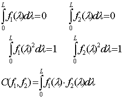 (1)
(1)
С value lies within the range of –1 to 1 and
features similarity of f1 and f2.functions. Such fi,
functions are selected out of all reference components which have the maximum С value.
Since among all spectral functions of the reference components there could be
no function sufficiently close to the studied spectral one the search is
limited by a minimum threshold value of Сmin. Should the
maximum found value of Сmax be less than this threshold, the substance would be
considered as unidentified (Смах is usually about 0.5-0.8 and is
chosen with regard to the video-signal quality and a number of reference
components). In case of the data is obtained from several hyperspectrometer
modules the resulting C value would be a weighted sum of correlations from these modules’ spectral functions:
 (2)
(2)
Here pi, is a weight of a
given module spectral function determined by informative capacity of the given
spectral range, m is a number of
hyper-spectrometer modules.
From the
mathematical viewpoint this method should be noted to be a particular case of
the more general sub-pixel transformation. It is similar to a product of two
vectors in multi-dimensional space and can be used for definition of each data
base element contribution, provided the basis formed by this base is
orthogonal. The correlation method undoubted advantage is its algorithmic
simplicity and high stability to interference caused by illumination and
various nonlinearities of equipment. The method’s drawback is its lower
information capacity of the obtained picture recognition for the hyper-spectral
survey results as compared sub-pixel method described below.
3.3.2.
Sub-pixel method for experimental data processing
All
superficial materials, as usual, are mixtures of several substances for all
measuring scales and, therefore, the spectral function of a surface image
element is a composition of several component spectral functions (reference
components). Modeling of each element spectral function by a linear combination
of a finite number of the reference spectral samples allows estimation of the
image pixel content by the least square method [1].
The
N-dimensional vector determined by N hyperspectrometer channels could be a
useful mathematic presentation for the spectral mixture analysis. An arbitrary
M reference spectral samples (while M always less than N) determines an
M-dimensional subspace in the N-dimensional vector space. We put the
N-dimensional vector of the image element spectral function as a linear
combination of reference vector components. Each component of the reference
spectral samples is defined by a numeric share value within 0 and 1. Besides,
the total sum of these numeric shares per each reference component of the given
image element must be equal to 1 with no account for noise and the unidentified
substances contribution. This geometrical interpretation of spectrum yields a
basis for the orthogonal subspace projections method (OSP) to analyze the mixed
spectrum.
The
reference components quantity depends on the spectral channels number, the
chosen spectral bandwidth, the spectral bandwidth signal to noise ratio, and
can vary from some few (in bad conditions) up to hundreds.
The essence
of sub-pixel elements recognition could actually be described as follows. As it
was mentioned above each image element is featured by its own spectral function
fi(l). Mind that
the sub-pixel transformation method brings fi spectral functions to
the same type as for the correlation method whereas their average value is zero
and the integral of square function is equal to 1 (1). In our case we deal with
discrete data and can denote such function as an intensity values series:
A={ fil1 fil2……..filn}, (3)
where filn is
intensity of the fi(l) spectral
function at the ln wavelength.
The sub-pixel transformation method presents this discrete function as a
N-dimensional vector with li (i=1 ¸ N) as the
coordinate axis.
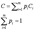
An example
helping to understand the sub-pixel method essence is the case when in a
hyperspectral image element spectral function (f) is characterized by three discrete values (lс, lк, lж) (Fig.1a).
|
Fig.1. |
Spectral function f, valued by three spectral channels (a), and its projection on
the reference components subspace |
Herein the
transformation uses the so-called linear mixing model. The model’s essence is
that each hyper-spectral image element represents a linear combination of
reference components with corresponding coefficients. So the studied f function is transformed to
where:
![]() is the vector presentation
for image element spectral function;
is the vector presentation
for image element spectral function;
![]() is the vector
presentation for reference components;
is the vector
presentation for reference components;
![]() is the vector
component contribution;
is the vector
component contribution;
![]() is the
reference components number;
is the
reference components number;
![]() is the error
vector caused by instrumental noises and unidentified substances;
is the error
vector caused by instrumental noises and unidentified substances;
![]() is a transposition operation.
is a transposition operation.
Expressions
(1) bring the spectra to vector type, and further on the obtained f vector is projected to a subspace
built-up by the reference components. The fп projection
and e perpendicular vectors to the
reference components subspace is a result of this procedure. It is obvious that
![]() (4).
(4).
Actually the perpendicular е vector is a
decomposition error due to insufficient number of the reference components. If
the f vector belongs to the
reference components vector subspace then the е error would
be zero, i.e. linear combination of the reference components vectors completely
describes the spectral function vector of the studied image element. The
decomposition error can be expressed by
![]() (5)
(5)
Since the
error vector is perpendicular to all reference components vectors the following
equation is valid
![]() (6)
(6)
where ST – is the transposed matrix. Using
(4) we get
![]() (7).
(7).
Transforming (7) finally yields
![]()
where ![]() is a reference components subspace projection matrix.
is a reference components subspace projection matrix.
Similarly
the error vector e can be obtained
using the PE error projection matrix
![]()
where ![]() , E is an identity matrix. The vector b coordinates (bi) give the
volume contributing by a particular i
– substance to the image pixel elementary content. The “error” vector value
reveals the actual validity of the taken reference components base to identify
the image pixel.
, E is an identity matrix. The vector b coordinates (bi) give the
volume contributing by a particular i
– substance to the image pixel elementary content. The “error” vector value
reveals the actual validity of the taken reference components base to identify
the image pixel.
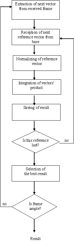
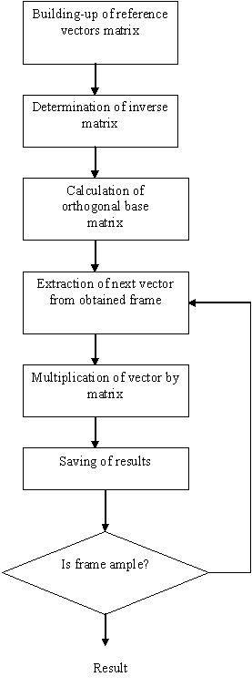
3.4.
Processing algorithms
Correlation method is
presented in the following figure:
Sub-pixel method is shown in
next figure:
4. Algorithms of initial configuring, routing, and reconfiguring
4.1. System composition
The complex
comprises a set of modules plugged in sockets on the system’s common
motherboard. On connection each module is assigned with its own unique
identifier. A part of the identifier is the socket number the module is plugged
in. We’ll give more details on the identifiers later. Let us consider
structures of the modules positioning and their interwork in the system.
Fig.2 gives
a diagram of physical connections between modules in the complex. Note that the
diagram depicts only module №004 connections with the modules concerned.
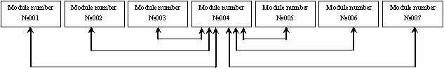
|
Fig. 2 |
Modules physical connections diagram |
All the
modules are instrumentally identical but differ only by functions they realize.
The functions are determined by software. Let us denote the different function
modules by the following abbreviations:
Rec is a data receiver. These modules
have external interface with the scientific equipment.
Proc is a module processing the
scientific data. These modules’ incoming data is processed according to the
module’s preloaded algorithm. The processed information is passed to transfer
modules.
Tran is a transmitter of data. The
module is responsible for the data transfer to outer devices.
Using the
notations the logical connections module diagram can be drawn this way:
![]()
|
Fig.3. |
The logical connections diagram for modules in case
of single module of a type |
If system
has a several similar function modules then the diagram could look as follows:
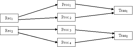
|
Fig.4. |
The logical connections diagram
for modules in case when number of modules executing each possible function
is more than one |
Therefore, each system module is
identified by the following parameters:
·
number of socket it is plugged in;
·
function fulfilled.
Assembly of these parameters is the
module’s identifier.
Operation of
the system needs each module to know the other module’s identifier to pass the
processed data to and the number of communication channel capable of making of
this transfer. The module connection diagram shows (Fig.1) that every module is
linked with other six modules via communication channels. These channels are situated
at the motherboard and in the common case, when not all the sockets are busy,
some communication channels could be lacking. So the first system start-up
stage must be initialization.
4.2.
Initialization stage
This stage
compiles a table according to which all the modules’ interwork takes place. Let
us call it a Routing Table.
Routing Table:
|
Row number |
Module Type |
Socket number |
Channel number |
|
1 |
Rec |
4 |
3 |
|
2 |
Proc |
2 |
2 |
|
… |
… |
… |
… |
The routing
table has the following fields:
Row number – as the table may include a
big number of different routes, each route represents a unique row in it.
Module type is the
assigned function of a module
Socket number is the
number of socket which the given module is plugged in.
Channel number is the number one of six
channels ready to carry data to a specified module. If the selected channel
links this module with the destination one indirectly, then a module that
received data addressed to another one transfers the information further
according to its routing table.
The table is generated this way. On system start-up each module sends a
broadcast request. This broadcast request includes the origin address, the type
mask of modules expected to answer, and parameter limiting the request’s “life
time”. Each module that received such a request must resend it via all its data
links. Each module satisfying the request mask must respond to the originator
with a message. This message contains the socket number that the given module
is plugged in and the type of the module. On reception of such a message the
broadcast request sender puts the message’s data into its own routing table.
The generated table may contain several records differed only by the “Channel
number” field value, this means presence of alternative routes to one and the
same module.
In order not to overload the system by such broadcast requests a
parameter is needed to limit its “life time”. This parameter is also included
into the requests. The parameter is a positive number decreased by one after
each request reception. If the resulted parameter value is not zero the request
is transferred forth. Thereby the number of the given request copies emerged in
the system is limited. This number is equal to 6n, where n is the parameter value, and number of
modules that received this request at least once equals to 6*n. Having
generated its routing table a module is switched to the operation mode.
4.3. Operation mode
In the operation mode a module can exchange data with other modules
according to the following scripts.
1. Data transfer to the module X
First a data
transfer request is originated. The request includes: the request-message
property, destination identifier, volume of data to transfer. On getting of the
data receive ready acknowledgement a data packet is formed and sent to the X
module. If no acknowledgement ever emerged then retry is made from the next
routing table raw that contains a route to the same type module as the X
module.
2. Data reception from the module X
On reception
of the data transfer request from X module a check is made for the input buffer
free space. If the buffer has enough space to receive the data the module sends
the data receive ready acknowledgement. After this the data packet from the X
module is received.
4.4. A module failure
If a module that has alternative modules of the same type fails the data
processing tasks would be redistributed among them. In this case the sender
will not get the data receive ready acknowledgement and the data is transferred
to some other module. The second consequence of the one module’s failure is a
loss of one data link for six other modules. Yet this trouble is surmounted by
using of alternative routes in the routing table. If not all system sockets are
occupied it would be better to place modules closer to each other. This gives
much stability as compared with modules spread over one or two sockets’
distance.
4.5.
Types of output data
After the
scientific data has been processed the system outputs three types of
information depending on the operation mode.
1)
Video-image (so called “raw data”)
This data is
taken from the optical system output and is practically unprocessed. The format
of this data is the following: the frame rate is 500 fps, the frame size is
1000х1000 pixels,
each pixel is one byte coded that provides for black & white image with 256
gray shades.
2)
Correlation technique results
These data
contain information on every spot of the studied surface as a complex of the
data base sample number and the similarity factor of the sample and the studied
spot spectral function. The data packet format is the following: the first 1
byte has the sample number and the second 1 byte is the similarity factor. So, the packet size is two bytes.
3)
Sub-pixel technique results
These data
contain information on every data base sample contribution value into the
studied surface section content. The data packet consists of Z contribution
factors for each sample. So, the packet size is Z bytes.
4.6.
Output data compression
Let us
estimate the compression efficiency for all three types of data. For comparison
we take two lossless compression techniques – LZW and Haffman method.
LZW-compression
replaces symbol strings with table codes. The Table is formed while processing
the input text. If the searched symbol string is found in the table the string
is then replaced with the string’s table index. Codes generated by
LZW-algorithm maybe of any length but they must have more bits then the single
symbol.
Haffman
compression replaces symbols with codes while the code length depends on the
frequency the symbol appears in the compressed data array. The technique
requires two passes through the array where the first pass counts the symbol
usage frequency and the second one makes the compression itself.
Programs
implementing the mentioned algorithms have been developed in order to test the
compression efficiency for different data types and each method. Ten 1MByte
arrays of each data type were used as the input data. The Table bellow gives
the averaged test results.
Table. Compression tests results:
|
|
Initial Size |
LZW compressed
size |
Haffman compressed
size |
|
Video-image |
1 MB |
1 006 000 Bytes |
696 000 Bytes |
|
Correlation data |
1 MB |
1 240 000 Bytes |
1 003 000 Bytes |
|
Sub-pixel data |
1 MB |
238 000 Bytes |
293 000 Bytes |
The Table
shows that the correlation processing data file is not compressed by the
algorithms discussed above, the sub-pixel processing data file is better
compressed by LZW method, and the video-image is better compressed by the
Haffman method.
References
1.
Vorontzov D.V., Orlov A.G., Kalinin A.P., Rodionov A.I., et al. Estimate of Spectral and Spatial Resolution for AGSMT-1
Hyperspectrometer, Institute of Mechanics Problems of RAS, Preprint №704
2. A.A.Belov, D.V.Vorontzov, D.Yu.Dubovitzkiy, A.P.Kalinin, V.N.Lyubimov,
L.A.Makridenko, M.Yu.Ovchinnikov, A.G.Orlov, A.F.Osipov, G.M.Polischuk,
A.A.Ponomarev, I.D.Rodionov, A.I.Rodionov, R.S.Salikhov, N.A.Senik,
N.N.Khrenov, “Astrogon-Vulkan” Small Spacecraft for High
Resolution Remote Hyper-Spectral Monitoring. Institute
of Mechanics Problems of RAS, Preprint №726