1             Introduction: class of problems under solution and structure of the algorithm

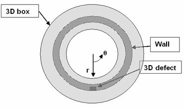
We consider a cylindrical pipe that can have a defect like a pit or hole. The cylindrical system of coordinates with the same axes as the pipe is used. It is supposed that defects are formed by set of hexahedral cells.

In order to avoid solution of a full external problem we subdivide it onto two stages. First the unperturbed two-dimensional field is calculated for the clean pipe (without defects) with a given geometry and excitation conditions. Than a three-dimensional subdomain (box) with the given defect is considered, and the three-dimensional problem for Maxwell equations with Dirichlet boundary conditions of the electrical field on the external boundaries is solved, see Figure 1 and Figure 2.

The two-dimensional unperturbed problem is solved by the algorithm described in [1]; so we have the solution for the azimuth component  of the vector potential of an axis-symmetric background solution. For the three-dimensional problem the electrical field  is represented in the box by sum of vector and scalar potentials

with the boundary values                                                             

.

It is supposed that the box is big enough to believe that the Dirichlet conditions from unperturbed problem can provide a required accuracy of modeling.

The three-dimensional problem in the box is solved by an iteration method (GMRES or MultiGrid algorithms, see Section 4) starting from the two-dimensional solution as an initial guess. Evidently this mixed (2D-3D) approach permits to drastically save computational efforts.

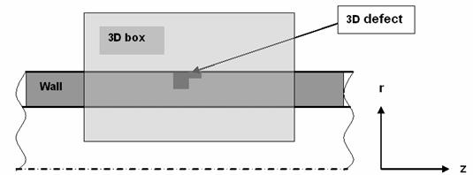
 Figure 1: Computational domain with the pipe wall,
cross-section at θ=const

Figure 2: Computational domain, cross-section at z=const

This work was supported by the RFBR grant No. 04-01-00567 and grant RM0-1298, CRDF.

2             Differential governing equations

The Maxwell equations written for the harmonic-in-time electromagnetic field () in media with a non-constant magnetic permeability , conductivity , and electrical permittivity   read

where  is a given source current density.

Numerical solution of these equations in three dimensions for media containing dielectric-ferromagnetic boundaries remains a challenge problem still. The known difficulties are discussed, e.g., in Introduction section of the paper [2], and we just remind two those important in our case:

·        handling regions of vanishing conductivity. The operator of the system has a non-zero kernel in these regions;

·        handling regions of strongly jumping conductivity and magnetic permeability at boundaries metal-air.

A more or less compromise approach to resolve the above mentioned issues consists of using a second order difference scheme on a staggered regular non-uniform grid to approximate the following corrected system of equations 

with auxiliary functions, and a constant, see details in the cited paper. 

This system is not the final one. It is possible to reduce the system to the second-order equations with 4 unknown scalar functions: three components of the vector potential and the scalar potential:

3             Difference scheme

In the cylindrical system of coordinates

our system of equations reads in the scalar form:

The three-dimensional solution is obtained in the computational domain (box)

for the whole azimuth angle . The box is covered by a structured grid having the hexahedral cells:

,

,

,

the number of cells is , , and   in , , and   directions, respectively.

We represent the computational domain by finite volumes with the central point corresponding to the index . Grid functions are defined on the following points referred to different faces and the center of the cell, respectively:

The cell centers with prescribed conductivity  and magnetic permeability  are calculated by

,

,

.

The corresponding difference equations on a non-uniform grid with spacing ,  and  read as follows:

          (2.1)

(2.2)

(2.3)

                 (2.4)

                 (2.5)

           (2.6)

(2.7)

                   (2.8)

                                                       (2.9)

                                                       (2.10)

                                                       (2.11)

(we give also the grid index for the right hand side of each equation).

Let us remove the half-integer indices by introducing notation

,

,

,

where superscripts “c” and “f” refer to the points located at the center and on a face of the cell, respectively; value of  μ  at the cell edges is evaluated by the arithmetic averaging, and  σ  at the cell faces is evaluated by the harmonic averaging.

The vector  of unknown difference functions consists of the four potential components:

                                                                                   (3) 

After some algebra, we exclude the functions ,  , and  from (2.1) to (2.11), and obtain the system of four difference equations:

We write the system of the algebraic equations for

as follows:

or in the matrix form

where  is a number of the unknown function (corresponds to the superscript of ),  is the equation vector number (number of the matrix row).

Let us describe the rules of forming the matrix entries. The calculation domain consists of , ,  cells along the coordinates  ,  ,  and , respectively. The rows of the matrix  and the right-hand-side vector  are calculated depending on the equation number , i.e. according to equations (4.1) to (4.4) if the index corresponds to an internal point, and according to the Dirichlet condition otherwise (other coefficients for ghost unknowns must be zero).

4             Solution of the difference system of equations  

The system of algebraic equations obtained after the discretization is really huge:  more than 250000 unknown complex values for a mesh of 40´40´40 cells (the typical mesh for a single simple defect). The system has a large conditional number because of a non-uniform grid and discontinuous coefficients on the metal-air boundaries. That is why finding of solution to this system is a difficult problem. Only iterative methods can be used. Here we consider use of GMRES with ILU preconditioning and Multigrid methods.

4.1           GMRES-ILU solver

The iteration Krylov subspaces method (GMRES algorithm) with an Incomplete Lower-Upper preconditioner is used by calling the correspondent procedures from the IMSL mathematical library. The solution procedure consists of two stages: calculation of the ILU factorization precondition matrix, and GMRES iterations with this preconditioner. The first stage requires large enough computational time comparing the iterations time: for instance 484sec versus 40sec. However, for the problem with multiple RHSs in (4.2), say N, one must calculate the preconditioner only once, and then it is used for iteration solution with each RHS. Hence the total computational time in this example equals 484 + N*40.

The main drawback of the GMRES-ILU approach consists of a large additional memory required by the ILU precondition matrix: in our computations the latter is usually at least 10 times greater than memory occupied by the matrix of the original system. This ILU matrix must be kept in computer memory. That is why there exists a limitation to the grid volume about 60´40´40 cells for the Windows PC (2 GB application memory). 

An optimal choice of the parameter Ω that drastically influence the number of iterations is Ω=0.5ω.

4.2           Multigrid algorithm

According to the original idea of the author of the multigrid method, see [3] to [6] the multigrid approach is based on the following observation. It is known that while exploring simple iteration methods the high-frequency components of the residual vanish much faster than the low-frequency ones. Therefore after several iterations on the initial fine grid, one can try to reduce the low-frequency part of the residual by using coarser grid. The coarser grid requires much smaller time for a single iteration and suppresses more efficiently the low-frequency harmonics.

Let us make general remarks concerning the efficiency of the multigrid method. Evidently it depends on all elements of the construction:

·        grid coarsening algorithm, “coarse” operators (matrices)

·        smoother strategy (operators  and numbers of subiterations )

·        restriction operators

·        prolongation operators

Additional difficulties for our case are caused by the following circumstances:

·        the staggered grids are used for difference equations; therefore the corner points of solutions at the metal-air frontiers do not match each other on the grids  

·        high contrasts in  influence strongly the choice of the smoother strategy.

However, theoretically the multigrid approach can provide a very efficient solution procedure for both memory and computational costs.

We consider the above listed elements in the subsections below.

Note that our current multigrid version permits to handle grids with 72´80´80 cells.

4.2.1               Generation of the “coarse” operators  

It is known that if we define the difference operator on a coarse grid by

                                                                                                        (5)

then it ensures the closeness of solutions on coarse and fine grids in the "weak", or "galerkin", sense. This choice of  is called Galerkin coarse grid approximation. The formula has theoretical advantages but its realization can be too computationally expensive in practice.

Another construction of the difference operator on a coarse grid is encountered in literature: the operator  is replaced by . It simplifies the realization significantly, yet its computational complexity is still very high.

An alternative method to obtain the coarse grid matrix  consists of a direct discretization of governing differential equations on the grid . This method is called discretization coarse grid approximation. The approach is quite simple and computationally cheap since the matrix coefficients are calculated by the same algorithm as for the fine grid. That is why we chose it currently.

Another source of different variants influencing the convergence rate originates from the possible structure of the matrixes  themselves. First of all, a rule of the unknown values  ordering in the one-dimensional vector  is critical. We have examined 14 different variants. Four of them are described by using construction of the implicit FORTRAN cycle:

A.   ,

B.   ,

C.   ,

D.   ,

The number of unknown values for the indexes  and  that correspond to  and  coordinates, respectively, is various for different function numbers  since some of them are referred to the centers of the grid cells and the others – to the faces. In case D, the variation limits of the function indexes are artificially set to be the same for all  by adding fictitious unknowns with correspondent identity equations. Otherwise the extra unknowns should be put to the end of the vector . This case has also been tested but it has no advantages over the case D.

A variant of modifying matrix  by eliminating the unknowns at the boundary points from the vector  has been examined separately. Such elimination is possible because the values  are explicitly defined at the boundary points (Dirichlet conditions). So the corresponding entries are put to the right-hand-side. One of the advantages of such modification is a noticeable reduction of the number of unknowns, especially for the coarse grids. For instance, in case of  grid cells in each direction, the number of difference equations is , the number of the boundary entries is about  (the condition of periodicity was taken into account earlier).

The following renormalization of matrix  rows gives an additional advantage while eliminating the boundary points: we multiply (4.1) by , (4.2) by , (4.3) by , and (4.4) by . Thus the solution of the system remains the same but the matrix  becomes symmetrical (the factor  provides independency of the matrix norms on the coarse/fine grid). The matrix symmetry property permits to double reduce the memory for matrix elements keeping.

4.2.2               The iteration methods (smoothers)

The smoothing methods in multigrid algorithms are usually chosen from the class of basic iterative methods. We are exploring the so-called two-layers iteration methods having the form

                                                                                       (6)

or

where  is the n-th iteration to the solution of the equation ,  is a preconditioner,  is the parameter of iterations, which is chosen from the condition of a fastest convergence.

Choice of the preconditioner is very critical.  The next two preconditioners have been constructed after analysis of the matrix  structure. Figure  shows a general fragment of  for the ordering variant A, see subsection 4.2.1, on a coarse grid  cells. The squares denote non-zero entries; the black squares belong to the main diagonal. One can observe that the density of the non-zero elements is sufficiently high at the three diagonals: main, and two neighboring. The remaining entries belong to diagonals that are separated by a distance from the main one, which grows while increasing the grid volume. That is why we take a simple preconditioner matrix having these three diagonals (with the minus sign). The matrix structure for the variants B and C is very similar. The matrix structure for the variant D is shown in Figure 4 (for the same grid volume). Now the non-zero entries occupy densely already nine diagonals: main, four above, and four below. Therefore a ninth-diagonal preconditioner matrix   has been examined in this case.

Figure 3: Non-zero entries of the matrix  (ordering variant A)

Figure 4: Non-zero entries of the matrix  (ordering variant D)

Below we describe some of the most important results (from our viewpoint) balking many others beyond the description.

The fastest convergence provides the three-diagonal preconditioner for the ordering A. The variant works about 10 times faster than the variant with the diagonal preconditioner (Jacobi method). The variant with the ninth-diagonal preconditioner has approximately the same number of multigrid cycles needed to diminish the residual  times as the three-diagonal variant. However, it requires more computational time per single iteration.

Important question is choice of values . We made experiments mainly for the two-grid algorithm with the three-diagonal preconditioners. A typical result for the clean pipe with the grid volume  is collected in Table 1.  Table cells contain total number of iterations for the fine and coarse grids (separated by the “plus” sign) that is needed to reduce the residual for  times; the total computational time is given as well.

Table 1

Solution of the same problem on a single grid requires 530 iterations and 23.4 seconds. Thus the two-grid method saves the computational time for about 4.5 times at =16 and =64. Note that the gain remains still enough if the parameters are significantly changed.

Similar results for the pipe with a groove defect (revolution symmetry) are collected in Table 2.  The grid volume is , residual drops  times. The single-grid problem requires 1822 iterations and 647 seconds. Thus the gain is about 16 times in computational time if =16 and =128.

Table 2

Optimization of parameters N1, N2, N3 for a three-grid method requires much more variants. We report the final result here for the same problem but another groove defect: 575, 52, and 23 seconds of computational time for single-grid, two-grid, and three-grid methods, respectively.

4.2.3               Restriction operators

At the moment we use coarse grids constructed by joining two cells along each direction. Speaking more precisely, eight grid cells of a fine grid with the same vertex are combined pair-wise in each direction into a single cell of the coarse grid.

All four unknown grid functions are referred to different points of the cell: the first three are referred to the centers of corresponding faces and the fourth one is referred to the cell center. Therefore individual interpolation formulas for each function are needed.

Consider the coarsening for one of the first three functions. The reduction is made consequently for each direction. As initial direction we take that corresponding to the considered function (function is referred to the center of faces orthogonal to the direction). The face coordinate of the coarse grid in this direction coincides with one of the face coordinate on the fine grid. Therefore the simplest way is to assign the function value on a fine grid to the function value on a coarse grid. However it is reasonable sometimes to filter the undesirable high-frequency component having the form of  where  is the point number along the considered direction. It is convenient to write the reduction as follows:

where  is the fine grid function,  is the coarse grid function,  is the coordinate along the considered direction. In order to exactly reconstruct linear functions, the coefficients  and  should be calculated by the following formulas:

The high-frequency component is filtered entirely at the value . The point-to-point transfer is done if , i.e. .

Along other directions the functions are referred to coordinates corresponding to the cell centers. The coarse cell center is located between the fine cell centers. Therefore either two-points linear interpolation or four-points cubic interpolation is explored.

The same consequent interpolation procedure is used for the fourth function.

Notice that the residuals are evaluated by different operators at the boundary and internal points. Therefore, the discrete function usually has a jump nearby the boundary (because of the Dirichlet conditions, the residual just vanishes at the boundary). Evidently, one cannot use the interpolation at the border points: an extrapolation from inner points is explored instead. It can generate unwanted perturbations.

4.2.4               Prolongation operators

Construction of the prolongation operators consists of subsequent linear or cubic interpolation for each direction.

An issue arises on the air-metal frontier because of discontinuity of the first derivatives in solution. Since we use a staggered grid, the points of discontinuity don’t coincide on fine and coarse grids. Therefore the prolongation operator generates undesirable perturbations of the residual in points nearby the frontier. One needs additional computational work on the fine grid to suppress these perturbations. Let us look at Figure 5 in order to illustrate the problem.

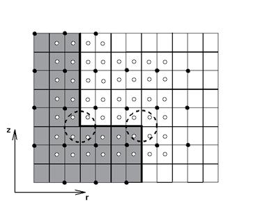
Figure 5: Coarse and fine grids

We show a two-dimensional cross-section  of the computational domain fragment.  The gray color denotes the subdomain occupied by the metal. Coarse and fine grid cells are drawn by thick and thin lines, respectively (each coarse cell joints four fine cells (eight in three dimensions)). The location of the azimuth component  considered on the coarse and fine grids is shown by the black and white circles, respectively. We see that these points do not coincide in the staggered coarse and fine grids (moreover black and white circles are also shifted in the direction normal to the sheet). Function  is not smooth near the metal-air boundary: it has the discontinuous derivative with respect to the normal direction. A typical one-dimensional graph along the direction is shown in Figure 6.

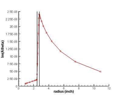
Figure 6: Imaginary part of  along radius at fixed.
Vertical lines denote the metal-air boundaries

Two typical two-dimensional graphs near the defect on the plane and plane are drawn in Figure 7 and Figure 8, respectively.

Therefore the prolongation operators, i.e. the evaluation of the correction function in the white circles from the values in the black circles (which is based on an interpolation procedure), can give and, in fact, does give “wrong” magnitudes near the boundary, especially in the corner regions shown by the dashed circles in Figure 5. 

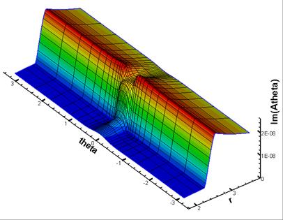
Figure 7: Imaginary part of  on the plane  corresponding to
the defect center

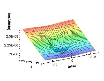
Figure 8: Imaginary part of  on the plane  corresponding to
the defect bottom face

The correction function prolonged from the coarse grid to the fine one has a wider domain of the singular behavior near the boundary (in terms of the number of cells).  During the multigrid cycle this implies the sharp growth of the local residual on the fine grid while adding the correction.

In order to overcome the issue we decided to make additional smoother iterations in the “singular” subdomains just after the prolongation operator. The correction function is changed locally in these subdomains (having several points width), and it becomes sharper near the air/metal boundary. Evidently this procedure is sufficiently computationally cheap, and it can be treated as a special kind of the interpolation correspondent to the solution structure. The procedure can be called the local smoother.

As to the way of interpolation, the preliminary observation is as follows: two-grid experiments show that the cubic interpolation has practically no advantage over the linear one. Moreover, it leads sometimes to instability of iterations. 

5             Example of calculations; modeling of the conical defect

In this example we consider the outer conical defect in the iron pipe with the wall thickness 8mm. The defect has 4mm depth, 16mm top diameter (on the wall surface) and 3mm bottom diameter.  This defect is located inside the uniform grid box of 8 r-cells, 16 -cells, and 16 z-cells. Each cell is considered as the “metal” one if it lies strongly outside the cone.  The “defect” box is a part of the whole non-uniform (r, ,z) grid having the volume of 56´80´80 cells. In Figure 9 the component  of electromagnetic field inside the pipe (surface , 5mm from the wall) near the defect is shown.

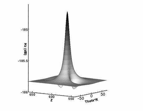
Figure 9: Conical defect: component  of EM field inside the pipe is mapped

In this example we use four grid levels. The graph of the residual history is shown in Figure 10. We stop the iterations after 15 MG cycles. Each MG cycle requires about 50 multiplications of the “main” matrix on the finest grid.  One can observe that the convergence rate is sharply drops after 11-th cycle. This is a typical behavior and we can not still overcome this effect. Note that already 10 MG cycles are enough in this example to obtain the solution with required accuracy.

Figure 10: Convergence history for 4 grid levels, the finest grid is 56´80´80

               Bibliography

         [1]     N. Zaitsev and Ivan Sofronov. “Method of calculating low-frequency electromagnetic problems in cylindrical geometry” Preprint of Keldysh Institute of Applied Mathematics, No. 61, 2004.

         [2]     Haber and U.M. Ascher, Fast finite volume simulation of 3D electromagnetic problems with highly discontinuous coefficients.  SIAM J. Sci. Comput. Vol. 22, No. 6, pp. 1943—1961, (2001)

         [3]     R.P. Fedorenko, “Introduction to the computational physics”, Moscow, MIPT, 1994, 526 pp.

         [4]     R.P. Fedorenko “Relaxation method for solving difference elliptic equations”, Jour. Comp.Math&Math.Phys., 1961, V.1, No.5

         [5]     R.P. Fedorenko, “About the convergence rate of an iteration method”,  Jour. Comp.Math&Math.Phys., 1964, V.4, No.3

         [6]     R.P. Fedorenko, “The iterative solution of the difference elliptic equations”, Adv. Math.Sci.,1973, V. 28, No.2