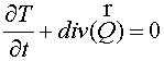
Аннотация
Рассмотрены различные численные методы для двумерных краевых задач для параболических уравнений.
Предполагается, что коэффициенты уравнений разрывны и линии разрывов не совпадают с
координатными. Это приводит к необходимости использования неортогональных сеток. Рассмотрены
полностью неявная, регуляризованная и аддитивные схемы. Специальный метод регуляризации,
учитывающий разрывы в коэффициентах, позволяет построить схемы более, чем первого порядка
аппроксимации по времени, которые легко распараллеливаются.
Abstract
The different computational methods for 2D parabolic boundary problems have been considered.
It is assumed the coefficients of the equations are discontinuous and the lines of
discontinuity don’t coincide with coordinate ones. It results in the necessity of using
the non-orthogonal grids. The fully implicit, additive and regularized schemes have been
developed. The specific method of regularization taking into account discontinuity of
coefficient allows constructing the schemes more than first order of time approximation,
which are easily parallelized.
Contents
1. Introduction
2. Fully implicit scheme
and support operator method
3. Regularized scheme
4. Finite difference flux method
5. Variational difference flux
method
6. Variational difference
locally one-dimensional method
7. Results of calculations
8. Conclusions
Reference
Introduction
Now there are many
difference schemes for the heat conductivity parabolic equations with
discontinuous coefficients, if the surfaces and lines of discontinuity being
not coincident with coordinate ones. The discontinuity of coefficients in a
heat conduction equation means that normal (to a discontinuity surface)
derivatives are discontinuous. In this case, attempts of approximating the
equations by means of the difference schemes without the taking into account
the position of discontinuities may reduce the accuracy of approximation. For
the best method of describing the phenomena it is expedient to use grids
adapted to the media structure. Besides the schemes should satisfy the
requirements of stability, monotonicity and conservativity. At the same time
because of the usage of multiprocessing systems, it needs to provide the
possibility of effective parallelezation of the difference schemes. But the
explicit schemes, most simply parallelized, are not considered because of hard
limitation of a time-step for schemes stability.
In the present work some methods of solution of the posed problem
for the 2D equation are considered
 , (1.1) , (1.1)
where
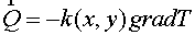 , (1.2) , (1.2)
in domain  . It is supposed that the coefficient . It is supposed that the coefficient  is a piecewise continuous
function. Boundary conditions may be general. The examined examples correspond
to zero boundary conditions of the second type is a piecewise continuous
function. Boundary conditions may be general. The examined examples correspond
to zero boundary conditions of the second type
 , (1.3) , (1.3)
where  is the boundary of
domain. Further, for simplicity we shall consider square
domain is the boundary of
domain. Further, for simplicity we shall consider square
domain  . .
The cells of examined grids have a
form of tetragons, though it should be noticed, that the proposed schemes might
be generalized easy for grids containing triangles. The well-known support
operator method has been used for a spatial approximation of the problem. The
feature of this method is a definition of the divergence and gradient
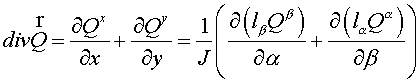
difference operators by using the difference analogy of the known identity:
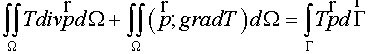 . (1.4) . (1.4)
If the operators of the divergence and gradient are in accordance with
the difference approximation of (1.4), the approximation orders of both
operators are matched.
Let  . The equality (1.4)
allows a definition of the divergence operator if the operator of gradient (or
the flux operator . The equality (1.4)
allows a definition of the divergence operator if the operator of gradient (or
the flux operator  ) is being determined. It is the reason of the method
denomination. Really, the support operator method approximates the system
(1.1), (1.2) instead of the approximation of the equation ) is being determined. It is the reason of the method
denomination. Really, the support operator method approximates the system
(1.1), (1.2) instead of the approximation of the equation  only. It is analogous to the ideas
developed in the known article (Glowinski R., Wheeler M.F., 1988). only. It is analogous to the ideas
developed in the known article (Glowinski R., Wheeler M.F., 1988).
Five difference schemes were
compared: fully implicit scheme on the basis of a of the support operators
method (Samarskii A.A., Koldoba A.V., Poveshchenko Yu.A., Tishkin V.V.,
Favorskii A.P., 1996; Koldoba A.V., Poveshchenko Yu.A., Popov Yu.P., 1985), the
scheme with regularizator (Samarskii A.A., 1989), two modifications for
curvilinear grids of the scheme proposed by Yu.B. Radvogin, and also a variant
of the locally one-dimensional scheme based on a variational-difference
principle (Goloviznin V.M., Korshunov V.K., Samarskii A.A., Chudanov V.V.,
1985). The results of comparison in midpoint of the process evolution and in a
final are represented in the tables.
The main aim of the article is to
create the effective methods of the 2D and 3D problems solution for the
parabolic equations with piecewise continuous coefficients. There are many
methods for rectangular grids but usually the surfaces and lines of the
coefficients discontinuity don’t coincide with coordinate ones. The parabolic
equations have standard forms of the balance equations connecting the time
derivatives of value with the flow divergence. The evident method is fully
implicit but it results in the solution of the linear system of the large
order. One possibility is determine the flow components at the intermediate
moments of the time and following divergent closure of the system. This idea
had been realized by Radvogin Yu.B. only for rectangular grids. The problem of
the mixed derivatives for nonrectangular grid had not been discussed in the
article. In this work it was shown that the contravariant component of flux
(DFM) or covariant components (VDFM) are sufficient to be calculated. Then
using the balance equation for each cell the divergence expression may be
obtained. The closed equations for the flux components may be constructed if
the mixed derivatives being omitted. The flux components equations are of the
order O(1). However, it is sufficient for the final approximation of the second
order for rectangular grid and of the first order for non-orthogonal grid.
Similar principles are used for VLODM. It is a sample of the additive scheme,
i.e. there is no approximation of each stage but only total.
The method considered is a
regularization method based on Samarskii idea analogous to preconditioning the
algebraic linear system. The difference approximation of the equations (1.1),
(1.2) may be rewritten  , where , where  , ,  , ,  and and  are finite difference
approximation of the operators by support operators method, are finite difference
approximation of the operators by support operators method,  and and  are positive
one-dimensional operators, described below. It is essential the scheme is
effective because it does not need to solve the complicated linear algebraic
equations, as the elliptic operator is determined on the explicit layer.
Besides, this scheme is easily parallelized. are positive
one-dimensional operators, described below. It is essential the scheme is
effective because it does not need to solve the complicated linear algebraic
equations, as the elliptic operator is determined on the explicit layer.
Besides, this scheme is easily parallelized.
The calculations for heat
conductivity coefficients with different analytical properties have been
realized for tasks on rectangular and curvilinear grids when the analytical
solution being known.
It is evident the proposed schemes may be generalized on a 3D
case.
Fully implicit scheme
and support operator method
Now we describe the most obvious
way of approximation: a fully implicit scheme and a method of operator  approximation. Let's mark, that
hereinafter the temperature is considered in cell-centers and corresponding
fluxes - in cell-edges. This method of discretisation allows the natural approximation
of boundary conditions of Neumann type. Besides, it simplifies the construction
of difference scheme near the surfaces or lines of coefficients discontinuities,
since the fluxes normal to these lines are continuous (it is supposed that
lines of discontinuities coincide with grid lines). approximation. Let's mark, that
hereinafter the temperature is considered in cell-centers and corresponding
fluxes - in cell-edges. This method of discretisation allows the natural approximation
of boundary conditions of Neumann type. Besides, it simplifies the construction
of difference scheme near the surfaces or lines of coefficients discontinuities,
since the fluxes normal to these lines are continuous (it is supposed that
lines of discontinuities coincide with grid lines).
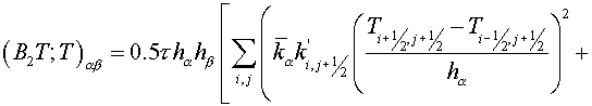
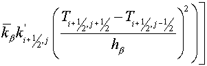
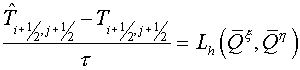
The fully implicit scheme has a
form
 (2.1) (2.1)
where  is a value is a value  on an implicit
time-layer, on an implicit
time-layer,  - difference approximation
of the operator - difference approximation
of the operator  by the support operator method. by the support operator method.
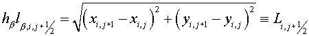
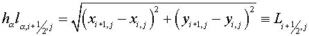
Support operators method is a version of the finite volume method. The
last one is based on the known identity 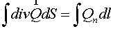 for a vector for a vector  . Thus it needs to know components of vector . Thus it needs to know components of vector  in the same points of cell
edges, but it is inconvenient, since the values of gradient different
components are usually determined in different edges. It is offered to average
the component values by usage of four neighbor bases (in a 2D case). Besides
the integral identity (1.4) will be used instead of the standard formulation of
the Gauss–Ostrogradskii theorem for calculating the divergence if the gradient
vector being known. The last one allows constructing a difference scheme not on
an initial grid, but on arbitrary one providing the best approximation. in the same points of cell
edges, but it is inconvenient, since the values of gradient different
components are usually determined in different edges. It is offered to average
the component values by usage of four neighbor bases (in a 2D case). Besides
the integral identity (1.4) will be used instead of the standard formulation of
the Gauss–Ostrogradskii theorem for calculating the divergence if the gradient
vector being known. The last one allows constructing a difference scheme not on
an initial grid, but on arbitrary one providing the best approximation.
The operator  was considered as the support
operator. Let was considered as the support
operator. Let  and and  be curvilinear
coordinates, under level lines passing through cell-centers or their corresponding
edges, and the distance between cell-centers for coordinates be curvilinear
coordinates, under level lines passing through cell-centers or their corresponding
edges, and the distance between cell-centers for coordinates  coincides with the
distance in coordinates coincides with the
distance in coordinates  . Besides it is
supposed, that under transformation . Besides it is
supposed, that under transformation  the domain the domain  is mapped into unit
square (see fig. 2.1). The numbers of a grid points along coordinate lines are
designated with is mapped into unit
square (see fig. 2.1). The numbers of a grid points along coordinate lines are
designated with  and and  accordingly. Then the covariant
components of a flux accordingly. Then the covariant
components of a flux  in local basis in local basis  look like look like
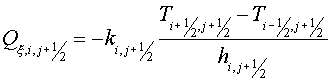 , (2.2) , (2.2)
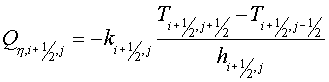 , (2.3) , (2.3)
 , (2.4) , (2.4)
 (2.5) (2.5)
 and
and
 are equal to the parts of segment are equal to the parts of segment
 and and 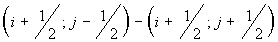 , lying inside a cell , lying inside a cell  , ,  and and  are the lengths of these segments. are the lengths of these segments.
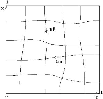
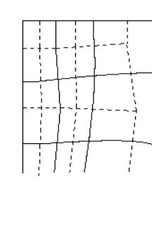
Fig.
2.1 Fig. 2.2
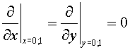
Suppose, that the grid lines are orthogonal to the boundary of the
domain (Fig. 2.1). Then we have according the boundary conditions (1.3)
  (2.6) (2.6)
For approximating the second term of the left hand part of (1.4) the
additional grid  has been constructed.
The edges of the grid has been constructed.
The edges of the grid  connect the cell
centers of the grid connect the cell
centers of the grid  . For covering of
whole area . For covering of
whole area  we shall add some cells formed
by segments of boundary and normals to it (see a fig. 2.2, the continuous lines
bound cells of a grid we shall add some cells formed
by segments of boundary and normals to it (see a fig. 2.2, the continuous lines
bound cells of a grid  , dashed - , dashed -  ). ).
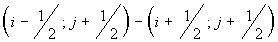
Let's consider an internal cell  of grid of grid  . Its vertices are denoted with F, G, H, I. The notation of angles is
represented in the fig. 2.3. Then the inner product of vectors . Its vertices are denoted with F, G, H, I. The notation of angles is
represented in the fig. 2.3. Then the inner product of vectors  and and  in the vicinity of vertex F has a form in the vicinity of vertex F has a form
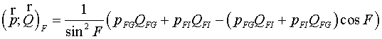 (2.7) (2.7)
Similarly in vertex G:
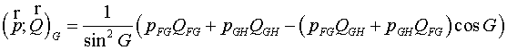 (2.8) (2.8)
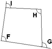
Fig. 2.3
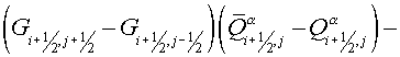
Using (2.6), (2.7) and analogous expressions for vertices H and I the
quantity of integral over the cell may be represented
 . (2.9) . (2.9)
Here  , ,  , ,  , ,  are some non-negative values,
the sum of which equals the square of FGHI. Let the vertices F, G, H, I have
indexes are some non-negative values,
the sum of which equals the square of FGHI. Let the vertices F, G, H, I have
indexes  , ,  , , 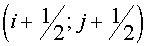 , , 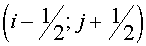 respectively. Then the expression (2.9)
may be rewritten respectively. Then the expression (2.9)
may be rewritten
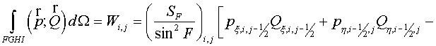 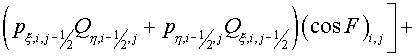  
 (2.10) (2.10)
For boundary cell, but not for an angular one, the sum (2.10) will
include only two terms. For example, for a cell  we obtain the following according
to (2.6): we obtain the following according
to (2.6):
 (2.11) (2.11)
For angular cells there will be only one term, which equals to 0 owing
to (2.6).
The integral over domain  , where summation is performed over all cells of , where summation is performed over all cells of  . .
Let grid vector  be a difference gradient: be a difference gradient:
 . It is possible to consider, that vector . It is possible to consider, that vector  component normal to boundary is equal to
0, i.e. component normal to boundary is equal to
0, i.e.   . .
Then
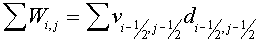 , (2.12) , (2.12)
Where  . .
Here for 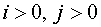
 (2.13) (2.13)

 (2.14) (2.14)
Remark, the sum (2.12) does not include expressions with  , that corresponds to boundary conditions (1.3). , that corresponds to boundary conditions (1.3).
Here  and and  are length of some segments. For
example, they may be the segments connecting centers of gravity of cells are length of some segments. For
example, they may be the segments connecting centers of gravity of cells  , ,  and and  , ,  of grid of grid  accordingly. Then it’s natural
to consider the expression accordingly. Then it’s natural
to consider the expression
 , (2.15) , (2.15)
as a difference analogue of the operator  , where , where  are squares of some domains,
associated with nodes are squares of some domains,
associated with nodes  . They may be squares of a tetragon with vertices in centers of gravity
of cells . They may be squares of a tetragon with vertices in centers of gravity
of cells  , ,  , ,  and and  of grid of grid  (it is assumed that for boundary
cells these vertices coincide with centers of boundary segments, and for
angular - with its angle vertex). It is possible to lie (it is assumed that for boundary
cells these vertices coincide with centers of boundary segments, and for
angular - with its angle vertex). It is possible to lie  for simpler variant. In fact it
means the theorem of Gauss-Ostrogradskii for this domain, and the grid
functions for simpler variant. In fact it
means the theorem of Gauss-Ostrogradskii for this domain, and the grid
functions  and and  are contravariant components of
a flux on cell edges of a grid are contravariant components of
a flux on cell edges of a grid  . .
The finite volume method was used in works of Edwards M.G. and
Aavatsmark I. for investigation of single-phase and multiphase problems of
underground hydrodynamics (M.G. Edwards, C.F. Rogers, 1998; Aavatsmark
I., Barkve T., O. Boe, T. Mannseth, 1996). They define the divergence using the
Gauss therem for one cell. The feature of the support operator method is a
definition of flux  from an equality (1.4). It results to the
following: the order of the divergence and gradient operators approximations is
the same. This method of difference schemes construction based on reviewing of
the system (1.1), (1.2) instead of the equation from an equality (1.4). It results to the
following: the order of the divergence and gradient operators approximations is
the same. This method of difference schemes construction based on reviewing of
the system (1.1), (1.2) instead of the equation 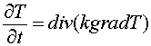 , that is similar to work Glowinski R., Wheeler M.F., 1988,
where the same representation is used for a mixed finite element method. , that is similar to work Glowinski R., Wheeler M.F., 1988,
where the same representation is used for a mixed finite element method.
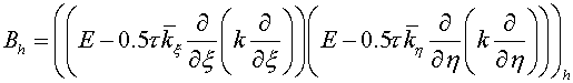
The regularized scheme
The following type of scheme is
developed as the regularized scheme:
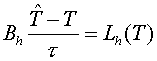 , (3.1) , (3.1)
where  operator is a
regularizator (Samarskii A.A., 1989). operator is a
regularizator (Samarskii A.A., 1989).
As known, for an absolute stability
of the scheme it is sufficient to examine
 (3.2) (3.2)
with boundary conditions
 (3.2 ') (3.2 ')
for the heat conductivity equation with a variable coefficient on a
rectangular grid (Samarskii A.A., 1989). Here  is a unit operator, is a unit operator,  is a max value of a
heat conductivity. The obtained scheme is a scheme of the first order of
approximation by time. Under drawing an analogy with rectangular grids it is
possible to use the regularizator of the following form for curvilinear grids is a max value of a
heat conductivity. The obtained scheme is a scheme of the first order of
approximation by time. Under drawing an analogy with rectangular grids it is
possible to use the regularizator of the following form for curvilinear grids
 (3.3), (3.3),
with boundary conditions
 (3.3 ') (3.3 ')
where  are curvilinear coordinates.
Coordinate lines of the system are curvilinear coordinates.
Coordinate lines of the system  coincide with lines of coordinates coincide with lines of coordinates  , but the initial grid maps into uniform rectangular one in a
plane , but the initial grid maps into uniform rectangular one in a
plane  with steps with steps  and and  (see fig. 2.1), (see fig. 2.1),  and and  are factors depending on "irregularity"
of a grid and for a rectangular grid equaling 1. are factors depending on "irregularity"
of a grid and for a rectangular grid equaling 1.
However, the regularizator of the type mentioned above gives
unsatisfactory results of calculations for the discontinuous coefficient of the
heat conductivity, as it does not provide the necessary order of the
approximation in the vicinity of the discontinuity line.
Because of this fact the following form of the regularizator  is offered: is offered:
  (3.4) (3.4)
with boundary conditions (3.3 ').
Usually regularized schemes are schemes of the first order of approximation
by time. The exception are the schemes on rectangular grids being the schemes
of the second order of approximation, if  and operators and operators  . Therefore it is possible to expect that the schemes of the type mentioned
above with regularized operators similar to main one of the problem near
coefficients discontinuity lines will be by more precise, than additive schemes
described below. . Therefore it is possible to expect that the schemes of the type mentioned
above with regularized operators similar to main one of the problem near
coefficients discontinuity lines will be by more precise, than additive schemes
described below.
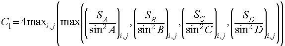
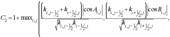
It is easy to find
expressions for factors  and and  , corresponding to absolute stability of the scheme (3.1)
with regularizator (3.4), for a concrete grid. Let , corresponding to absolute stability of the scheme (3.1)
with regularizator (3.4), for a concrete grid. Let  be a grid function,
obtained on be a grid function,
obtained on  -th time step ( -th time step ( ). Under stability the following will be understood ). Under stability the following will be understood
 (*) (*)
Here is an inner product in the space of grid functions, defined in
cells of a grid  (the summation is performed over
all cells of a grid (the summation is performed over
all cells of a grid  ): ):
 (3.5) (3.5)
as well as
 (3.5’) (3.5’)
It should be noted that it needs to introduce last terms in both parts
of (*). It is concerned with the fact the expressions in the (*) without terms
are not a norms, but just as semi-norms. So the left part is a norm in solution
space and right part is a norm in space of initial data.
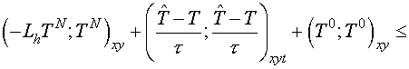
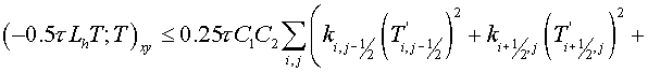
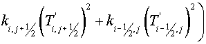
Let's prove, that the satisfaction of the inequality
 . (3.6) . (3.6)
is sufficient for
stability of the scheme (3.1) (in sense of (*)).
Really, having multiplied both parts of (3.1) by  (in inner product (in inner product  ), we have: ), we have:
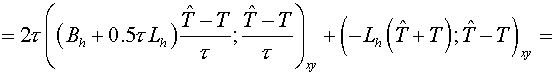
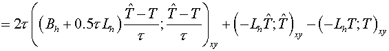
Thus, if (3.6) is
fair, then 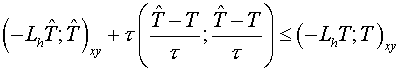 , from which (*)
immediately follows. , from which (*)
immediately follows.
Besides the inner product  we shall introduce we shall introduce
 , ,
where the summation is performed over all cells of a grid  . It should be marked, that norms induced by inner products . It should be marked, that norms induced by inner products  and and  are equivalent: are equivalent: 
Then,
 , (3.8) , (3.8)
 , (3.9) , (3.9)
 . (3.8) . (3.8)
and
 (3.10) (3.10)
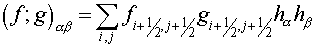
Here 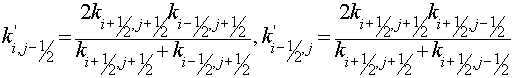
For approximation of 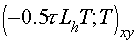 it is assigned in (1.4) it is assigned in (1.4)  just as it was done in support
operator method. Then the right part of (1.4) becomes 0 and according to the
formulas (2.13), (2.14) just as it was done in support
operator method. Then the right part of (1.4) becomes 0 and according to the
formulas (2.13), (2.14)
 , (3.11) , (3.11)
where 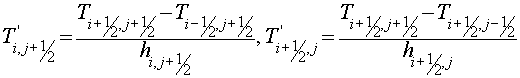 , and the summation is performed over all cells of a grid , and the summation is performed over all cells of a grid  . .
Thus,
 , (3.12) , (3.12)
where
Since each edge appears twice in the sum (3.12) except the boundary
ones, it is sufficient to suppose
 (3.13) (3.13)
 (3.14) (3.14)
for satisfaction of 
Let's assume  . Then both introduced inner products coincide and it is necessary to
prove . Then both introduced inner products coincide and it is necessary to
prove 
 , where , where  , ,
 with boundary conditions (1.3).
Since both operators with boundary conditions (1.3).
Since both operators  are non-negative determined
(with respect to inner product are non-negative determined
(with respect to inner product  , which coincides with , which coincides with  in a considered case), all their
eigenvalues in a considered case), all their
eigenvalues  , corresponding to eigenfunctions , corresponding to eigenfunctions  , are non-negative. Consider the case , are non-negative. Consider the case  . Since all grid functions are decomposed by basis . Since all grid functions are decomposed by basis  : :  , then , then
 . .
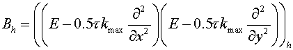
Thus, we have proved, if having selected regularizing factors according
to the formulas (3.13) and (3.14) the scheme (3.1) will be absolutely stable.
As several tests without analytical solution have shown it will be also stable
for variable  . In other cases the regularizator (3.3) should be used. . In other cases the regularizator (3.3) should be used.
It should be noted, that for the considered class of problems the scheme
(3.1) with  equal to squares of tetragons
with vertices in center of gravity of cells equal to squares of tetragons
with vertices in center of gravity of cells  , ,  , ,  and and  of grids of grids  , was also absolutely stable (with some , was also absolutely stable (with some  and and  ). Moreover, the scheme (3.1) with regularizator of the form ). Moreover, the scheme (3.1) with regularizator of the form
 (3.15)
with boundary conditions
 (3.15') (3.15')
was absolutely stable for some
 and
and
 . .
Let's remark, that the scheme (3.1) with regularizator (3.4) or (3.15)
is economic, since the corresponding system of linear equations may be easily
inverted by two sweep methods.
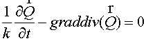
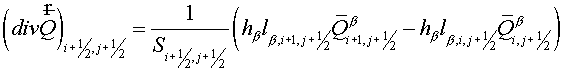
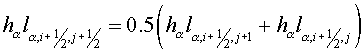
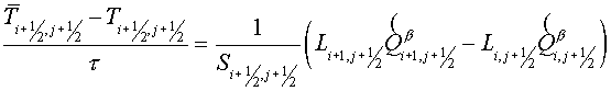
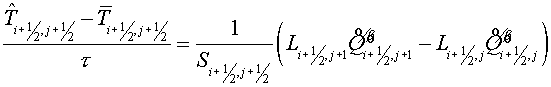
Difference flux method
Flux method is understood as the
scheme of following sort: at the first step (predictor) the fluxes on edges of
cells are calculated on "a intermediate time layer using the equations for
each component of a vector  . Usually they are difference approximations of the equation
for a flux . Usually they are difference approximations of the equation
for a flux  by some methods. The
second step (corrector) is a divergent closure due to initial equation. by some methods. The
second step (corrector) is a divergent closure due to initial equation.
Let's remind the scheme proposed by
Yu.B. Radvogin for a heat conductivity equation with variable coefficient on a
rectangular uniform grid.
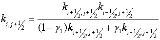
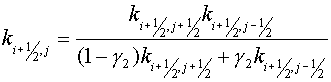
Predictor
 (4.1) (4.1)
 (4.2) (4.2)
Corrector
 (4.3)
(4.3)
Here  and and  are grid steps, are grid steps,  and and  are fluxes normal to
the cell edges. If are fluxes normal to
the cell edges. If  the scheme is
absolutely stable, i.e. the scheme with surpassing definition of fluxes is
stable. the scheme is
absolutely stable, i.e. the scheme with surpassing definition of fluxes is
stable.
On a step of predictor we
effectively calculate components of fluxes normal to the cell edges referred to
intermediate time layer. It should be noted, that each equation of (4.1) and
(4.2) approximates equation for a flux with zero order, i.e. it is supposed
that for each layer of cells the flux through its lateral boundaries is equal
to zero. On a step of corrector using these values we calculate values of
temperature for an implicit time layer.
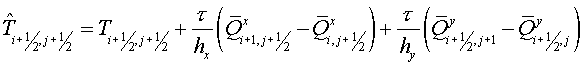
The natural generalizing for
curvilinear grids of the scheme proposed by Yu.B. Radvogin looks like the
following:
predictor
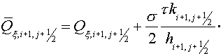
 (4.4) (4.4)
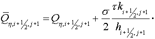
 (4.5) (4.5)
Here  is defined by support
operators method for each layer along directions is defined by support
operators method for each layer along directions  and and  under the following
assumption. It is supposed that flux along the same direction in other layers
and flux along other direction are equal to 0. under the following
assumption. It is supposed that flux along the same direction in other layers
and flux along other direction are equal to 0.
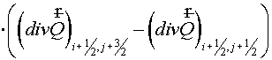
Corrector
 (4
.6)
(4
.6)
The operator  is defined by a
support operator method: using contravariant components of a flux we calculate
the covariant ones by a method depicted above. The equations (4.4) and (4.5)
also may be solved effectively. is defined by a
support operator method: using contravariant components of a flux we calculate
the covariant ones by a method depicted above. The equations (4.4) and (4.5)
also may be solved effectively.
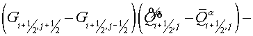
Variational difference flux method
Let the operator  be employed to both parts of (1.1) and then outcome be
multiplied by be employed to both parts of (1.1) and then outcome be
multiplied by  . Then due to (1.2) the equation for flux is obtained . Then due to (1.2) the equation for flux is obtained
 (5.1) (5.1)
Discretising in time with the help
of the implicit scheme ( ), we have ), we have
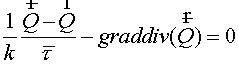 (5.2) (5.2)
Multiplying (5.2) by an arbitrary
variation  and integrating over
arbitrary domain and integrating over
arbitrary domain  we obtain due to
boundary conditions (1.3), if boundary fluxes being equal to zero: we obtain due to
boundary conditions (1.3), if boundary fluxes being equal to zero:
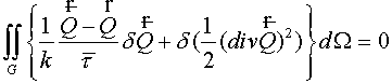 . (5.3) . (5.3)
Thus, functional
 (5.4) (5.4)
reaches its stationary value on a solution of the equations (1.1) and
(1.2) with boundary conditions (1.3).
Let the curvilinear coordinates  in domain in domain  be
introduced by the same way as in the third item. For a definiteness we suppose
that a Jacobian be
introduced by the same way as in the third item. For a definiteness we suppose
that a Jacobian  . Designating . Designating  and and  number of cells along
directions number of cells along
directions  and and  respectively, the
expressions in (5.4) may be rewritten in local contravariant base of a curvilinear
coordinate system respectively, the
expressions in (5.4) may be rewritten in local contravariant base of a curvilinear
coordinate system  . .
The orts of contravariant base look
like
 , (5.5) , (5.5)
where  are Lame coefficients
of a curvilinear coordinate system. are Lame coefficients
of a curvilinear coordinate system.
Since  , ,
where  and and  are contravariant
components of flux then having made substitution are contravariant
components of flux then having made substitution  we obtain we obtain
  , (5.6) , (5.6)
 . (5.7) . (5.7)
As well as in a difference flux
method, we suppose that for each layer of cells the flux through its boundary
is equal to zero. Let's consider the approximation of a functional (5.4),
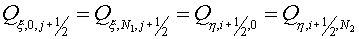
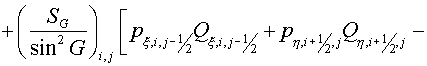
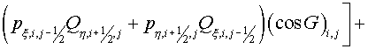
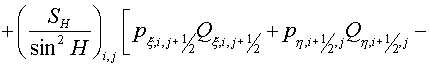
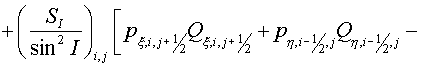
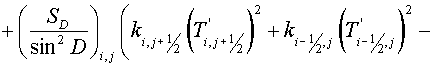
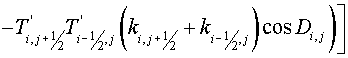
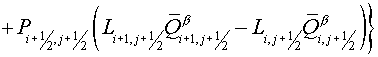
having taken into account of any layer of cells along  or or  as as  (see fig. 5.1). (see fig. 5.1).
For a layer  along along  we have: we have:
 , (5.8) , (5.8)
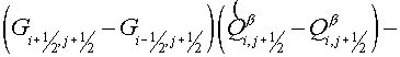
where
 (5.9) (5.9)
 (5.10) (5.10)
 (5.11) (5.11)
 (5.12) (5.12)
 (5.13) (5.13)
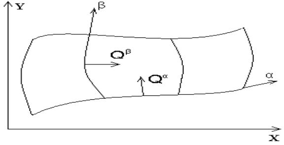
Fig. 5.1
Then functional  may be represented as may be represented as
 , (5.14) , (5.14)
where
 , (5.15) , (5.15)
 . (5.16) . (5.16)
The difference analogue of the
equation (5.1) follows from a condition of a minimum of a functional (5.8):  or or
 (5.17) (5.17)
Using boundary conditions  the equation is
solved by sweep method. the equation is
solved by sweep method.
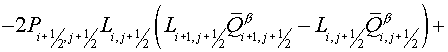
For a layer  along along  the reasonings are
similar, therefore we list only finite outcome - difference equation: the reasonings are
similar, therefore we list only finite outcome - difference equation:
 (5.18) (5.18)
and boundary conditions  . .
For divergent closure we use the
initial equation (1.1) and formula (5.7):
 . (5.19) . (5.19)
The variational locally one-dimensional method
The developed scheme is very
similar with previous one. Let's specify their differences. In a flux method
using known distribution of temperature the fluxes on an intermediate time
layer are calculated, and then divergent closure is performed. In the given
scheme using known temperature covariant component of a flux only along one
direction (for example, along  ) is calculated, then the temperature on an intermediate time
layer is obtained under supposition that the fluxes along ) is calculated, then the temperature on an intermediate time
layer is obtained under supposition that the fluxes along  are equal to zero.
Then using the new distribution of temperature on an intermediate time layer
covariant component of a flux along are equal to zero.
Then using the new distribution of temperature on an intermediate time layer
covariant component of a flux along  is calculated.
Finally, the temperature on an implicit time layer is obtained under assumption
that of a component of the flux along is calculated.
Finally, the temperature on an implicit time layer is obtained under assumption
that of a component of the flux along  is zero. Since the
calculations coincide with one described above we represent only final formulas
– the difference equations: is zero. Since the
calculations coincide with one described above we represent only final formulas
– the difference equations:
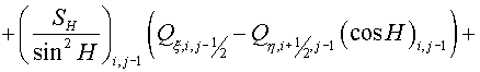
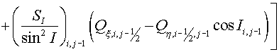
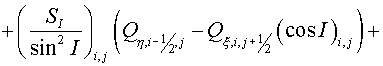
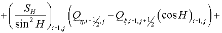
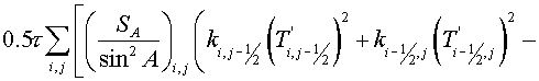
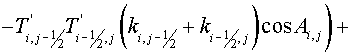
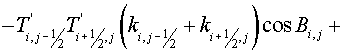
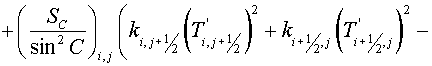
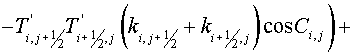
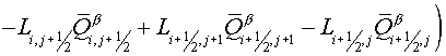
 (6.1) (6.1)
 (6.2) (6.2)
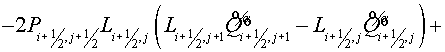 (6.3) (6.3)
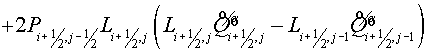
 (6.4) (6.4)
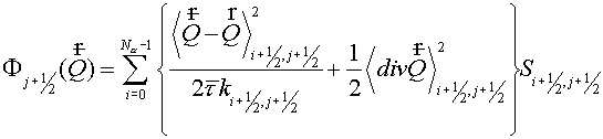
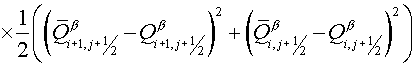
Calculation results
All five algorithms were tested on
a rectangular grid, scalene grid (see fig. 7.1) and sine grid (see fig. 7.2).
The square  was divided into 10х10, 20х20 and 40х40 of cells. The exact solutions were the
following was divided into 10х10, 20х20 and 40х40 of cells. The exact solutions were the
following
1. 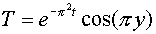 , , 
2. 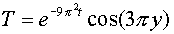 , , 
3. 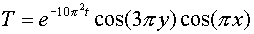 , , 
4. 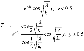 , , 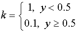 , ,
where  is obtained from the
equation is obtained from the
equation
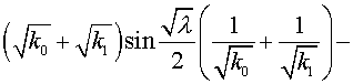 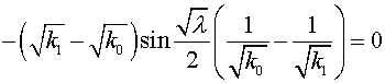 (7.1) (7.1)
Besides, the problem with sources
have been tested too. Instead of (1.1) the following equation have been
considered  . At the same time
the regularized and fully implicit schemes have been developed. These schemes
were also tested on solution . At the same time
the regularized and fully implicit schemes have been developed. These schemes
were also tested on solution
5. 
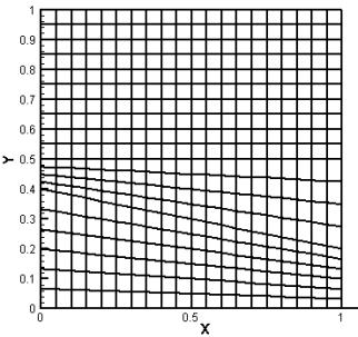 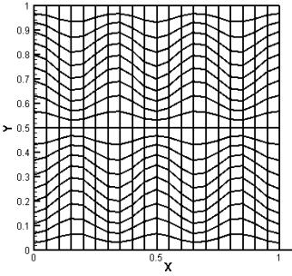
Fig. 7.1 Fig. 7.2
|
|
The
middle of calculation
|
Final
moment
|
|
Rectang.
|
Scalene
|
Sine
|
Rectang.
|
Scalene
|
Sine
|
|
10
|
Implicit
|
0.002543
|
0.005791
|
0.017498
|
0.004267
|
0.004786
|
0.005831
|
|
Regul.
|
0.001028
|
0.005610
|
0.018306
|
0.001701
|
0.002891
|
0.004672
|
|
DFM
|
0.003288
|
0.009470
|
0.044702
|
0.005555
|
0.006121
|
0.007731
|
|
VDFM
|
0.003288
|
0.006604
|
0.015847
|
0.005555
|
0.005988
|
0.006746
|
|
VLODM
|
0.003288
|
0.006745
|
0.017656
|
0.005555
|
0.006006
|
0.006412
|
|
20
|
Implicit
|
0.001802
|
0.002757
|
0.003224
|
0.003002
|
0.003170
|
0.002974
|
|
Regul.
|
0.000255
|
0.002479
|
0.002564
|
0.000419
|
0.001269
|
0.001628
|
|
DFM
|
0.002562
|
0.014380
|
0.068315
|
0.004299
|
0.004519
|
0.008980
|
|
VDFM
|
0.002562
|
0.003858
|
0.009687
|
0.004299
|
0.004412
|
0.004330
|
|
VLODM
|
0.002562
|
0.003945
|
0.010538
|
0.004299
|
0.004419
|
0.004205
|
|
40
|
Implicit
|
0.001614
|
0.001661
|
0.001674
|
0.002684
|
0.002732
|
0.002675
|
|
Regul.
|
5.910e-5
|
0.001393
|
0.001048
|
9.692e-5
|
0.001078
|
0.001036
|
|
DFM
|
0.002378
|
0.037927
|
0.043497
|
0.003983
|
0.005954
|
0.006813
|
|
VDFM
|
0.002378
|
0.003501
|
0.003585
|
0.003983
|
0.003988
|
0.003924
|
|
VLODM
|
0.002378
|
0.003427
|
0.003743
|
0.003983
|
0.003990
|
0.003912
|
Table 7.1
|
|
The
middle of calculation
|
Final
moment
|
|
Rectang.
|
Scalene
|
Sine
|
Rectang.
|
Scalene
|
Sine
|
|
10
|
Implicit
|
0.060256
|
0.084513
|
0.052579
|
6.954е-9
|
0.003246
|
7.405е-4
|
|
Regul.
|
0.035828
|
0.066245
|
0.034633
|
1.694e-9
|
0.004266
|
0.001353
|
|
DFM
|
0.076859
|
0.099951
|
0.093450
|
1.642е-8
|
0.003478
|
7.715е-4
|
|
VDFM
|
0.076859
|
0.100001
|
0.064092
|
1.642е-8
|
0.003300
|
0.001186
|
|
VLODM
|
0.076859
|
0.100644
|
0.062796
|
1.642е-8
|
0.003302
|
0.001289
|
|
20
|
Implicit
|
0.042323
|
0.049574
|
0.039917
|
2.493е-9
|
7.776е-4
|
9.130е-5
|
|
Regul.
|
0.016587
|
0.024491
|
0.021972
|
4.006e-10
|
0.001244
|
4.014е-4
|
|
DFM
|
0.059831
|
0.069960
|
0.087101
|
6.660е-9
|
9.922е-4
|
1.112е-4
|
|
VDFM
|
0.059831
|
0.066459
|
0.058264
|
6.660е-9
|
8.126е-4
|
6.367е-4
|
|
VLODM
|
0.059831
|
0.066603
|
0.058629
|
6.660е-9
|
8.135е-4
|
6.438е-4
|
|
40
|
Implicit
|
0.037857
|
0.039757
|
0.037575
|
1.895е-9
|
1.930е-4
|
4.612е-6
|
|
Regul.
|
0.011800
|
0.015915
|
0.017438
|
2.436e-10
|
6.094е-4
|
1.101е-4
|
|
DFM
|
0.055590
|
0.062290
|
0.072428
|
5.273е-9
|
4.033е-4
|
5.492е-6
|
|
VDFM
|
0.055590
|
0.057125
|
0.055641
|
5.273е-9
|
2.220е-4
|
1.999е-4
|
|
VLODM
|
0.055590
|
0.057186
|
0.055720
|
5.273е-9
|
2.223е-4
|
2.004е-4
|
Table 7.2
|
|
The
middle of calculation
|
Final
moment
|
|
Rectang.
|
Scalene
|
Sine
|
Rectang.
|
Scalene
|
Sine
|
|
10
|
Implicit
|
0.058951
|
0.080214
|
0.038918
|
9.32е-10
|
0.002992
|
2.058е-4
|
|
Regul.
|
0.033464
|
0.060647
|
0.042225
|
1.762e-10
|
0.004628
|
2.669е-5
|
|
DFM
|
0.058421
|
0.077163
|
0.055781
|
9.03е-10
|
0.003042
|
1.950е-4
|
|
VDFM
|
0.058421
|
0.079921
|
0.045288
|
9.03е-10
|
0.003015
|
2.455е-4
|
|
VLODM
|
0.066577
|
0.087797
|
0.048211
|
1.468е-9
|
0.003015
|
2.640е-4
|
|
20
|
Implicit
|
0.043829
|
0.050063
|
0.040376
|
3.47е-10
|
7.128е-4
|
1.048е-5
|
|
Regul.
|
0.017012
|
0.024025
|
0.020200
|
4.493e-11
|
0.001601
|
3.104е-5
|
|
DFM
|
0.043922
|
0.051174
|
0.065077
|
3.49е-10
|
7.568е-4
|
2.731е-5
|
|
VDFM
|
0.043922
|
0.050462
|
0.045016
|
3.49е-10
|
7.251е-4
|
3.991е-5
|
|
VLODM
|
0.052266
|
0.058096
|
0.050214
|
5.93е-10
|
7.254е-4
|
4.490е-5
|
|
40
|
Implicit
|
0.040019
|
0.041671
|
0.039675
|
2.68е-10
|
1.760е-4
|
4.102е-7
|
|
Regul.
|
0.012873
|
0.016171
|
0.015776
|
2.893e-11
|
8.474е-4
|
7.318е-6
|
|
DFM
|
0.040273
|
0.048669
|
0.055690
|
2.72е-10
|
2.191е-4
|
6.596е-6
|
|
VDFM
|
0.040273
|
0.042710
|
0.042085
|
2.72е-10
|
1.856е-4
|
9.758е-6
|
|
VLODM
|
0.048662
|
0.050290
|
0.050019
|
4.69е-10
|
1.864е-4
|
1.131е-5
|
Table 7.3
|
|
The
middle of calculation
|
Final
moment
|
|
Rectang.
|
Scalene
|
Sine
|
Rectang.
|
Scalene
|
Sine
|
|
10
|
Implicit
|
0.029916
|
0.139758
|
0.111295
|
0.068440
|
0.132269
|
0.068473
|
|
Regul.
|
0.027471
|
0.143325
|
0.117483
|
0.062569
|
0.126339
|
0.071540
|
|
DFM
|
0.031644
|
0.139261
|
0.118225
|
0.072636
|
0.136601
|
0.066644
|
|
VDFM
|
0.031644
|
0.143370
|
0.119056
|
0.072636
|
0.137619
|
0.070704
|
|
VLODM
|
0.031644
|
0.144451
|
0.117742
|
0.072636
|
0.137898
|
0.071240
|
|
20
|
Implicit
|
0.010815
|
0.152431
|
0.024321
|
0.022945
|
0.056930
|
0.016478
|
|
Regul.
|
0.008049
|
0.153958
|
0.021091
|
0.017029
|
0.051391
|
0.012137
|
|
DFM
|
0.012768
|
0.147452
|
0.068678
|
0.027176
|
0.060852
|
0.021627
|
|
VDFM
|
0.012768
|
0.155467
|
0.025705
|
0.027176
|
0.061600
|
0.021214
|
|
VLODM
|
0.012768
|
0.157788
|
0.025298
|
0.027176
|
0.061783
|
0.021195
|
|
40
|
Implicit
|
0.005784
|
0.097919
|
0.006320
|
0.012025
|
0.028871
|
0.011572
|
|
Regul.
|
0.002941
|
0.096378
|
0.003688
|
0.006122
|
0.023593
|
0.006318
|
|
DFM
|
0.007790
|
0.092611
|
0.042937
|
0.016247
|
0.032853
|
0.017442
|
|
VDFM
|
0.007790
|
0.098255
|
0.008891
|
0.016247
|
0.033321
|
0.015941
|
|
VLODM
|
0.007790
|
0.100245
|
0.008740
|
0.016247
|
0.033407
|
0.015942
|
Table 7.4
|
|
The
middle of calculation
|
Final
moment
|
|
Rectang.
|
Scalene
|
Sine
|
Rectang.
|
Scalene
|
Sine
|
|
10
|
Implicit
|
8.242е-5
|
8.480е-5
|
6.975е-4
|
0.010368
|
0.010438
|
0.014873
|
|
Regul.
|
2.162e-5
|
2.398e-5
|
4.494e-5
|
3.519е-4
|
3.905е-4
|
0.001466
|
|
20
|
Implicit
|
2.250е-5
|
2.959е-5
|
8.245е-5
|
0.002562
|
0.002585
|
0.002981
|
|
Regul.
|
2.452е-5
|
2.536e-5
|
2.656e-5
|
9.644e-5
|
1.422е-4
|
2.441е-4
|
|
40
|
Implicit
|
4.942е-6
|
9.133е-6
|
6.943е-6
|
6.071е-4
|
6.142е-4
|
6.127е-4
|
|
Regul.
|
2.552e-5
|
2.574e-5
|
2.532e-5
|
6.182e-5
|
7.687e-5
|
7.351e-5
|
Table 7.5
The results of calculations are
represented in tables 7.1…7.5 according to number of the test (1…5). Final time
for tests 1…4 was 0.25, for the test 5 was  . Numbers of steps by time are 100 and 600 respectively.
Factors . Numbers of steps by time are 100 and 600 respectively.
Factors  and and  are supposed to be
equal to 1.5 in the scheme with regularizator (3.15). are supposed to be
equal to 1.5 in the scheme with regularizator (3.15).
Conclusions
The computer simulation of the different
boundary and initial problem demonstrates some features of the methods
developed. All additive and almost additive schemes DFM, VDFM, VLODM have the
same accuracy and CPU times. The fully implicit scheme accuracy is better than
for additive scheme but CPU time is essentially more and there is a serious
problem of parallelelizing this scheme. The best scheme is a regularized one.
The error of the approximation and CPU time are less than for other methods
except the case of the large values of function decrements. Besides the order
of the time approximation is more than the first as it has been discussed
above.
If the spatial part of the function is  and the decrement is and the decrement is  the asymptotic stability of the scheme is not
satisfied. Really at the end of evolution the absolute error of the solution is
1.694e-9 for rectangular grid, 0.00426 for scalene grid and 0.00135 for
sinusoidal one, if the step is about of 1/10. For N=20, 40 correspondingly the
values of errors are 0.00124, 6.094e-4 for scalene grid. As for other methods
the error were less. It may be explained by the fact that regularization
operators are not strictly agreed with the approximation of the elliptic
operator by the support operator method. the asymptotic stability of the scheme is not
satisfied. Really at the end of evolution the absolute error of the solution is
1.694e-9 for rectangular grid, 0.00426 for scalene grid and 0.00135 for
sinusoidal one, if the step is about of 1/10. For N=20, 40 correspondingly the
values of errors are 0.00124, 6.094e-4 for scalene grid. As for other methods
the error were less. It may be explained by the fact that regularization
operators are not strictly agreed with the approximation of the elliptic
operator by the support operator method.
Author expresses thank to Pergament
A.Kh. for proposed topic of investigation and invaluable assistance during
article preparation.
Reference
1. Samarskii
A.A. The theory of difference schemes. Moscow, “Nauka”, 1989 (in Russian).
2. Samarskii
A.A, Koldoba A.V., Poveshchenko Yu.A., Tishkin V.V., Favorskii A.P. Difference
schemes on irregular grids. Minsk, 1996. (in Russian)
3. Goloviznin
V.M., Korshunov V.K., Samarskii A.A., Chudanov V.V. The method of factorized
heat displacements for solution of 2D problems of heat conductivity on
irregular grids. Preprint of KIAM, N58, 1985 (in Russian).
4. Glowinski
R., Wheeler M.F. Domain decomposition and mixed finite element methods for
elliptic problems. - First
International Symposium on Domain Decomposition Methods for Partial
Differential Equations, Philadelphia, 1988, SIAM, pp.144-171
5. Edwards
M.G., Rogers C.F. Finite volume discretisation with imposed flux continuity for
the general tensor pressure equation. Computational geosciences, vol 2, 1998,
pp 259-290
6.
Aavatsmark I., Barkve T., O. Boe, T. Mannseth.
Discretisation on non-orthogonal, quadrilateral grids for inhomogeneous
anisotropic media. Journal of computational physics, 127, 1996, pp 2-14
|