Spectral nonlocal boundary conditions for the wave equation in moving media
Preprint, Inst. Appl. Math., the Russian Academy of Science

Нелокальные спектральные граничные условия для волнового уравнения в движущейся среде

Introduction

The considered wave equation for the moving media occurs after the formal change of variables

                                                                                                   (1.1)

in the wave equation

                                                                               (1.2)

where  is a given constant speed,  is the speed of sound, . It reads

                            .                     (1.3)

Here is the axis looked to the right in the global (rest) coordinate system, and  is the similar axis in the local system of coordinates uniformly moving to the left. The latter system is usually associated with the body (wing) immersed in the uniform flow.

Equation (1.3) describes propagation of the perturbations of the pressure or the velocity potential and can be immediately obtained from the Euler equations linearised about the uniform flow, cf. [Sofronov-JMAA] .

In order to numerically simulate acoustic waves governed by (1.3) high-order finite volume or finite difference methods are used. These methods require “non-reflecting” boundary conditions on open boundaries such that they could have really small reflections*. At least the error arising because of spurious reflections should not be greater than the approximation error in the interior. One of the best choices is exact (transparent) boundary conditions. The correspondent operators have been obtained and implemented for the wave equation in case of , spherical boundary, see [Sofronov-DAN] , [Sofronov-EJAM] , [Grote-Keller SIAM]  , [Hagstrom-AN] , and in case of , channel, see [BBS-AIAA] . In both cases a spectral approach is used to derive analytically the desired operators of the boundary conditions. Namely the Fourier method on the open boundaries: spherical functions or imaginary exponentials for 3D or 2D spherical boundary, and cosines for inflow/outflow cross-sections of the channel, respectively.  The larger number of the basis functions being taken into account the higher accuracy of a discrete counterpart (i.e. smaller amount of reflections). Each Fourier coefficient – which is a function of time and the normal spatial variable – is treated separately by recurrence formulae with respect to time.

Possibility of use of the Fourier method is a key feature in the construction of the abovementioned operators of boundary conditions. Evidently this spectral approach permits to tune the accuracy of required discretization to the approximation error in the interior. In both spherical and plain cases the Fourier method was used owing to the fact that the governing equations have uniform coefficients on the transversal coordinate surfaces: spherical or polar coordinates for Eq. (1.2) outside 3D/2D sphere, and Cartesian coordinates for Eq. (1.3) in the channel to the left from the inflow cross-section and to the right from the outflow cross-section, see Figure 1, shaded regions extended to infinity (white regions correspond to computational domains).

Figure 1 : Spherical (left) and plain-channel (right) geometries

 

Unfortunately an immediate treatment of Eq. (1.3) with  in the spherical geometry, see Figure 1 left, by the spectral approach similar to the case of  –  what is very desirable for the aeroacoustics in open domains – is not possible because of variable coefficients with respect to the azimuth angle: the Fourier method does not work. In this paper, we propose a way to find an approximate solution to this challenge. Idea consists of using a discrete counterpart of the problem from the beginning with successive derivation and efficient approximation of the “spectral” boundary operator in terms of a discrete Fourier basis.

The outline of the paper is as follows. In Section 1 we formulate the problem, the two-dimensional case is considered for simplicity (polar coordinates). Section 2 describes main steps of the algorithm of generating boundary conditions correspondent to the homogeneous case of zero velocity , a bridge to the inhomogeneous case  is made. The latter is considered in Section 3. Numerical examples demonstrating accuracy of the approach are given in Section 4.  Section 5 contains several conclusions.

Note that idea to use discrete governing equations outside domain of interest was proposed by V. S. Ryaben’kii and it has been explored, in particular in [RTT-JCP]  to construct non-local ABCs for 3D wave equation. A principal discrimination of this and our approaches consists of ways of approximations of obtained operators that originally require too large computational resource.

The method [RTT-JCP]  is based on the property of 3D wave equation to have lacuna, while our approach develops approximation of boundary operator by sum-of-exponentials. The latter is more generic from the view of applications; at least we can treat 2D wave equation where the method [RTT-JCP]  does not work.

1.    Problem formulation and governing equations

We omit the prime in Eq. (1.3) hereafter for a convenience, and restrict ourselves by the two-dimensional case; the approach is generalized straightforwardly for the three-dimensional case as well.

Let us consider Cauchy problem for the equation

                                      (2.1)

supposing that exciting data functions are concentrated inside a finite domain:

The original problem consists of constructing artificial boundary conditions ABCs on  such that waves propagate through  without reflection.

A disk with a radiusis taken here as the domain:

.

Remark. As usual in formulation of problem of generating ABCs one needs to point exactly the governing equations outside  only. Consequently the aim is to replace these governing equations by proposed ABCs. No concretization of equations inside  is required as a rule.

We introduce the polar coordinates

                                                                                 (2.2)

and rewrite (2.1) in the form:

   (2.3)

Equation (2.3) or more precisely some its difference counterpart outside the disk  will be the main equation in our analysis.  The desired “low-reflecting” boundary conditions will be generated numerically.

We will need also a simple local boundary condition for (2.3) on . To generate it let us take the well-known condition

for the 2D wave equation and make the change of variables (1.1) . After some algebra, putting  in the time-dependent coefficients, we obtain the desired local condition:

                                                   (2.4)

2.    Case a=0

We reproduce here main elements of the approach [Sofronov-EJAM] of generating analytical transparent boundary conditions for the Eq. (2.3) , . This will be a background to make a generalization for the case .

Let us consider first the following auxiliary extended IBVP for a function  on

                                                                         (3.1)

Here  is the basis of imaginary exponentials on ,  is the Dirac’s delta function.

The problem has analytical solution expressed in the form

                                                          (3.2)

where  is the modified Bessel function (see for example [A-S] ), denotes the inverse Laplace transform .

Evidently, the solution  of the IBVP with arbitrary Dirichlect boundary data ,

                                                                              (3.3)

is written down as

                                                                                     (3.4)

where  denotes convolution with respect to the time variable, and  are the Fourier coefficients defined from the decomposition of

on the boundary .

Notice that the convolution kernel  is written in the factorization from

                                                                           (3.5)

with

Coming back to the interior IBVP we propose to use (and we do use) the formula (3.4) to calculate function on the open boundary while developing a numerical algorithm for solving the reduced problem in . Let us clarify this on the example of an explicit difference scheme. Denote by  last three -grid points of the polar mesh in . Suppose the solution is already known for the time-layers with . Then using a second-order finite-difference scheme one can update the solution on the  time layer for all  points except the boundary point . The solution at point  is calculated by (3.4) taking Dirichlect data at  as . Figure 2 schematically represents the algorithm. Thus we obtain the transition operator from the layer  to the .

It is important to emphasize that the convolution kernel  is handled by the sum-of-exponentials approximations:

This representation allows the recursive evaluation of the convolution operator in (3.4) and dramatically reduces; see details in [Sofronov-EJAM] .

Figure 2:  Schematic representation of the update algorithm.

3.    Case a>0

Now consider the equation (2.3) for . Similarly to (3.1) we have the following auxiliary IBVP

                                                                           (4.1)

where  denotes the wave operator (2.3) in moving media.

Auxiliary “elementary” kernels

Evidently there is no simple analytical formula for the solution in this case. Therefore let us consider the discrete counterpart for (4.1) :

                                                                          (4.2)

I.e. we introduce the polar grid in

and suppose that we are able to calculate solution of (4.2) - grid function  with . The details of the finite-difference scheme will be discussed below.

Evidently we have  discrete problems (4.2) since the discrete basis on  consists of  discrete functions .

First, similarly to (3.3) we consider the discrete problem

                                                                            (4.3)

with arbitrary Dirichlect data . Its solution can be expressed in terms of the solution :

                                                                             (4.4)

where  are the Fourier-coefficients of  in the basis , i.e.

and  denotes the discrete convolution  operator defined by the following rule

Next we introduce the “elementary” kernels  which are the Fourier-components of  in the basis  numerated so that

                                                                           (4.5)

here  can have the values .

The following matrix notation clarifies the formula (4.5)

               (4.6)

Remark. In case  owing to the separation of variables the matrix in (4.6) is diagonal, i.e.  if , cf. (3.5) .

Each elementary kernel depends now on temporal index  only (at fixed radial index ).

Thus (4.4) can be rewritten in the form

                                                     (4.7)

Formula (4.7)  will serve us to generate low-reflecting boundary conditions, cf. (3.5) .

Numerical aspects of the algorithm

At first we say some words about the finite-difference scheme for (2.3). All derivatives are approximated by central second order finite differences. The scheme is implicit in time because of the mixed derivatives and at each time step we have to solve the linear system , where  is a solution on the current time step . Matrix  has the form , where  is the identical matrix,  corresponds to the  derivatives,  corresponds to the  derivatives. To inverse the matrix  we use the simple iterations in form

with ,  is  approximation of ,  is an iterative parameter. On each iteration step we have to inverse two three-diagonal matrices that are handled by the sweep method.

We define the basis  by imaginary exponentials on the equidistant grid:

.

Discrete delta function  is given simply by

According to (4.7) we must calculate the kernels  for all time steps  such that , where  is a calculation time. However, similarly to the update algorithm shown in Figure 2, it is enough to keep functions  only for single value of . Nevertheless these calculations of “elementary” kernels in (4.6) are very expensive. It requires also large memory resources to keep  as well as large computational costs to calculate the convolution in (4.7) .

That is why we have developed set of modifications to (4.7) in order to sharply reduce the computational costs. First we subdivide the passing waves onto low and high frequencies (with respect to spatial grid size). Therefore we decrease the summation limits in (4.7) . Only low-frequency harmonics with  are treated accurately with the non-local discrete boundary condition. For high-frequency harmonics, discretization of the local boundary condition (2.4) is used. The new limits correspond to the truncation of the matrix , i.e. instead of  matrix we consider  matrix.

Next we introduce restriction on the summation index : let  belong to the interval  simply throwing away any others .

We will see in the examples of numerical simulation that such approximations of the full matrix in (4.6) do have a sense: it is sufficient to take small enough  to produce accurate results.

Thus we really need only a band submatrix  in (4.6) :

Finally, and this is the most valuable modification to reduce computational costs, we use a technique developed in [AES-CMS]  and approximate each discrete convolution kernel by sum of exponentials:

                                           (4.8)

here  is the power in the last term.

This representation allows for the recursive evaluation of the convolutions in (4.7) .

In practice we use  for large enough computational time and therefore we need calculate in advance and keep only about  complex numbers to represent each “elementary” kernel. So the cost of our approximation to (4.7) is not too large: more exactly the requirements on memory are estimated by  of real values and the computational cost is estimated by  operations per time step, .

Incorporation of the modified formula (4.7) into a difference scheme for interior problem in order to update solution at the external open boundary is made in the same manner as described in the previous section. The only discrimination is that we must treat a band matrix of “elementary” kernels (width) instead of simply diagonal one (the parameter)

According to the algorithm described in [AES-CMS]  the approximation (4.8) can be obtained by knowledge of  at . Thus the extended auxiliary problems are computed only for several first time steps.

4.    Numerical examples

In order to avoid singularities in the origin we consider the annular domain . We impose homogeneous Dirichlect boundary conditions at  and our discrete non-local boundary conditions at . The velocity  and .

Two equidistant meshes are used: coarse one with , and fine one with .

In the simulations we consider the equation (2.3). The initial data is taken to zero and the source is introduced as a right-hand side in equation (2.3) having the form

Here  is so-called Ricker signal with the central frequency , see Figure 3 (left)

the source distribution is on Figure 3 (central) with

and the frequency dependence of the source is on Figure 3 (right)

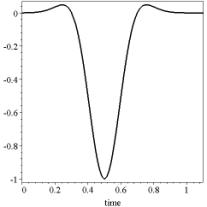
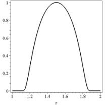
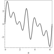
Figure 3: time dependency, Ricker function (left); distribution on r variable (central); -distribution (right).

We compare calculated solutions with the reference solution  obtained on the extended area  and on the very fine mesh so that this discrete solution can be identified with the exact.

Below we represent the results in continuous norm  measured over our annular domain . Note that the errors for -norm have the same orders and behavior.

In Figure 4 (top) we represent the relative errors of the solutions  obtained on the extended areas, i.e. the errors that are due to the approximations of the difference scheme on our grids.

Then in Figure 4 (bottom) we represent the relative error of the solutions  with low-reflecting boundary conditions in form (4.7) compared with the solution computed on the extended domain on the same mesh. We set  for the coarse mesh and  for the fine one. The results are pretty well: “boundary” errors are much less than the approximation errors (20 to 30 times) and don’t affect the resulting error.

Note that if we use the local boundary condition (2.4) at  then the errors have the values compared with the solution, i.e. the errors are about 100%.

The demonstrated results confirm that  can be small enough compared to . In Figure 5 - norm of  in logarithm scale is shown. We take here -norm is calculated with respect to , correspondent to 5 seconds. One can observe a sharp peak near .

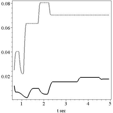
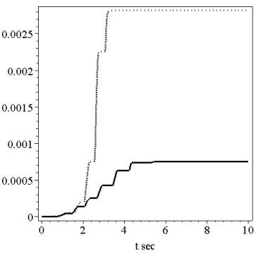
Figure 4: relative errors of the solution calculated on extended domain, dashed line is for the coarse mesh (), solid line is for the fine mesh (). Top figure corresponds to the reference discrete solution on the extended region:

, bottom to the solution with our boundary condition at :

We summarize the influence of the parameters  on relative errors in the tables below. Table 1 results correspond to the coarse mesh, Table 2 to the fine one.

The reader can compare these values with those on the Figure 4, right:  coarse and  fine grids, respectively.

Table 1: Relative errors for the coarse mesh for the different sizes of the matrix  band.

Table 2: Relative errors for the fine mesh for the different sizes of the matrix  band.

It is impotent to notice that we use the approximation representation (4.8) to reconstruct the kernels  for  where  is large enough. According to the algorithm for finding coefficients  in (4.8) we need function on a short time interval only, i.e. , where . Of course such construction is not correct for arbitrary medium. For example it is obvious that we cannot apply such procedure for the medium with some inhomogeneous in some distance from the external boundary. But our medium has no obstacles and we don’t expect some impulse arrived from outside.

Another difficulty with usage of (4.8) occurs while considering large values of . If   is small enough the kernel looks like one presented in Figure 6 (top.). Such kernels are approximated very well by the sum-of-exponentials (4.8) . But if  increases the kernel becomes like one from Figure 6 (bottom). It is impossible here to construct the approximation (4.8) with decaying exponentials at short time. Fortunately for the case of our coarse and fine meshes we don’t need to deal with such “bad” kernels. Pretty well accuracy is achieved without considering kernels of these types.

If we need finer meshes we must consider “bad” kernels as well. Let us discuss two possible ways how to avoid the difficulties with the approximation.

Evidently the nature of this oscillation behavior is owing to the delta-function Dirichlect boundary data while calculating the elementary kernels, see (4.2) . Therefore the first way is to work with submeshes. I.e. we can try to find the kernels on finer sub meshes with smooth ”delta” functionoriginated from the main grid. Thus the kernels will be smoother and could permit desired approximations. The second way consists in using more sophisticated finite-difference scheme in (4.2) that gives smaller oscillations for discontinuous initial data.

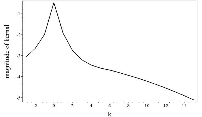
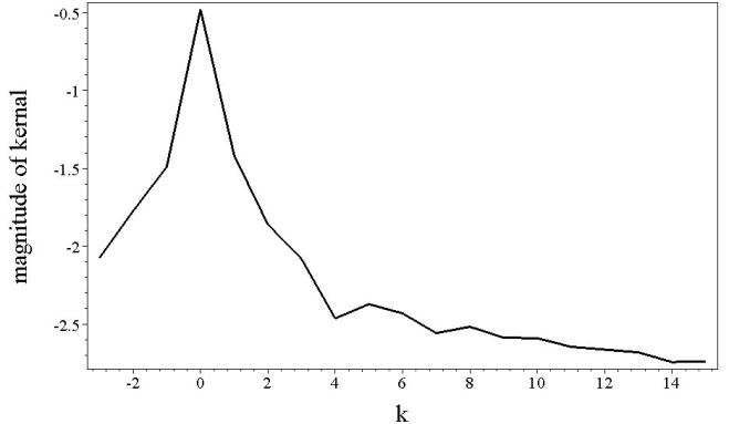
Figure 5: - norm of , , versus distance . Velocity a=0.2  (top) and a=0.7 (bottom).

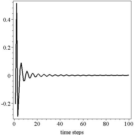
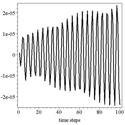
Figure 6: Amplitude of “elementary” kernels  for ;  (top) and  (bottom).

5.    Conclusions

In this paper we have introduced the novel approach of constructing discrete transparent boundary condition for the wave equation in the moving media. Necessary approximation modifications of exact formula leading to low-reflecting boundary conditions are proposed. These modifications permit to rapidly calculate the boundary operator. Numerical examples show that the error due to reflections is much less than the error due to finite-difference scheme.

Also the described algorithm may be considered as a generic method to construct low-reflecting boundary conditions for the different kind of equations and boundary shapes. We already have some results concerning the wave equation in the layered media and we think about another applications.

As mentioned above there are some open questions while approximating the kernels. They required more detailed investigation and this will be a part of our future work.

References

[Sofronov-JMAA] Sofronov, I. L. Non-reflecting inflow and outflow in wind tunnel for transonic time-accurate simulation, J. Math. Anal. Appl., V. 221, (1998) 92—115.

[Sofronov-DAN] Sofronov, I. L. Conditions for complete transparency on a sphere for the three-dimensional wave equation, Russ. Acad. Sci. Dokl. Math. Vol. 46, No.2 (1993) 397—401.

[Sofronov-EJAM] Sofronov, I. L. Artificial boundary conditions of absolute transparency for two- and three-dimensional external time-dependent scattering problems, Euro. J. Appl. Math., V.9, No.6 (1998) 561—588.

[Grote-Keller SIAM]  M.J.Grote and J.B.Keller, Exact nonreflecting boundary conditions for the time dependent wave equation, SIAM J.Appl.Math. 55 (1995), 280-297.

[Hagstrom-AN] T.Hagstrom, Radiation boundary conditions for the numerical simulation of waves,

Acta Numerica 8 (1999), 47-106, Cambridge: Cambridge University Press, 47-106.

[BBS-AIAA] Ballmann J.;  Britten G.; Sofronov I. Time-accurate inlet and outlet conditions for unsteady transonic channel flow, AIAA Journal, Vol. 40 (2002), No. 2., 1745—1754.

[RTT-JCP] V. S. RYABEN'KII, S. V. TSYNKOV, AND V. I. TURCHANINOV, Global Discrete Artificial Boundary Conditions for Time-Dependent Wave Propagation, J. Comput. Phys., 174 (2001) pp. 712-758.

[A-S] 1. Abramovitz M., Stegun I. A. Handbook of Mathematical Functions, National Bureau of Standards, Applied Math. Series #55. Dover Publications, 1965.

[AES-CMS] Arnold A; Ehrhardt M.; Sofronov I.  Discrete transparent boundary conditions for the Schroedinger equation: Fast calculation, approximation, and stability, Comm. Math. Sci. 1 (2003), 501-556.