Introduction:
short description of the 3D algorithm
In [1] we have proposed a
numerical method of calculating harmonic three-dimensional electromagnetic
field in the metallic pipes with local defects. The goal of the present paper
is to describe the modifications of the algorithm which allows computing fields
around relatively small or complex defects.
In this section we give short
description of the initial algorithm.
We consider one or several
coaxial cylindrical pipes that can have defects like pits or holes. For the
simplicity we will consider the case of a single pipe, although the algorithm
permits to compute the case of several coaxial pipes. The cylindrical system of
coordinates with the same axes  as the pipe(s) is
used. It is supposed that the defects can be approximated by a set of
hexahedral cells. as the pipe(s) is
used. It is supposed that the defects can be approximated by a set of
hexahedral cells.
In order to avoid solution of
a full external problem we subdivide it onto two stages. First the unperturbed
two-dimensional field in the domain

is calculated for the clean
pipes (without defects) or for the pipes with 2D defects (which do not depend
on the azimuth angle) with a given geometry and excitation conditions. Then a
smaller three-dimensional subdomain (box)

with the given defect is
considered, and the three-dimensional problem for Maxwell equations with
Dirichlet boundary conditions of the electrical field on the external
boundaries is solved, see Figure
1 and Figure
2.
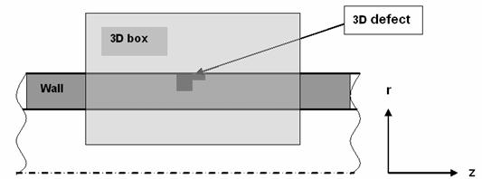
Figure 1. Computational domain, cross-section at θ=const
The two-dimensional
unperturbed problem is solved by the algorithm described in [2]; so we
have the solution for the azimuth component  of the vector
potential of an axis-symmetric background solution. For the three-dimensional
problem the electrical field of the vector
potential of an axis-symmetric background solution. For the three-dimensional
problem the electrical field  is represented in the
box by sum of vector and scalar potentials is represented in the
box by sum of vector and scalar potentials

with the boundary
values
 . .
It is supposed that the box is
big enough to believe that the Dirichlet conditions from unperturbed problem
can provide a required accuracy of modeling.
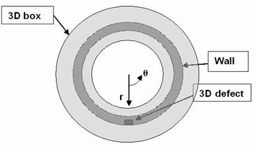
Figure 2. Computational domain, cross-section at z=const
The three-dimensional problem
in the box is solved by the multigrid iteration method starting from the
two-dimensional solution as an initial guess.
In order to overcome the known
difficulties with kernel of the Maxwell equations, see, for example, [3], we
use the following modified Maxwell equations written for the fixed frequency ( ) in media with a non-constant magnetic permeability ) in media with a non-constant magnetic permeability  , conductivity , conductivity  , and electrical permittivity , and electrical permittivity
 : :

where  is a given source
current density, is a given source
current density,  is an auxiliary
function, and is an auxiliary
function, and  is an auxiliary
constant, see details in the cited paper. is an auxiliary
constant, see details in the cited paper.
This system is not the final
one. It is possible to reduce the system to the second-order equations with 4
unknown scalar functions: three components of the vector potential  and the scalar
potential and the scalar
potential  : :


We write the system
of the algebraic equations in matrix form for the vector of unknowns
 , ,
where

as
follows:

or

where  is a number of the
unknown function (corresponds to the superscript of is a number of the
unknown function (corresponds to the superscript of  ), ),  is the equation vector
number (number of the matrix row). is the equation vector
number (number of the matrix row).
The system has a large
conditional number because of a non-uniform grid and discontinuous coefficients
on the metal-air boundaries. That is why finding of solution to this system is
another difficult problem. We have observed that the multigrid algorithm is a
most effective one in both computational time and memory. In [1] we described
our implementation of the multigrid method applying to the problem. In
particular, we decided to make additional smoother iterations in the “singular”
subdomains just after the prolongation operator. The correction function is
changed locally in these subdomains (having several points width), and it becomes
sharper near the air/metal boundary. Evidently this procedure is sufficiently
computationally cheap, and it can be treated as a special kind of the
interpolation correspondent to the solution structure. The procedure can be
called the local smoother.
The rest of the paper we
devote to computing electromagnetic fields in cases of small, multiple, or
complex defects. Namely, we discuss ways to safe required computational
resources: some “technical” tricks and so called embedded grids approach.
2 Increase of grid volume of solving problems
There exists a limitation to
the grid volume for the Windows PC (2 GB application memory). That is why we
made additional efforts to increase the possible grid volume which can be
processed using PCs.
A variant of modifying matrix  by eliminating the
unknowns at the boundary points from the vector by eliminating the
unknowns at the boundary points from the vector  has been examined.
Such elimination is possible because the values has been examined.
Such elimination is possible because the values  are explicitly defined
at the boundary points (Dirichlet conditions). So the corresponding entries are
put to the right-hand-side. One of the advantages of such modification is a
noticeable reduction of the number of unknowns, especially for the coarse grids
of the multigrid algorithm. For instance, in case of are explicitly defined
at the boundary points (Dirichlet conditions). So the corresponding entries are
put to the right-hand-side. One of the advantages of such modification is a
noticeable reduction of the number of unknowns, especially for the coarse grids
of the multigrid algorithm. For instance, in case of  grid cells in each
direction, the number of difference equations is grid cells in each
direction, the number of difference equations is  , the number of the boundary entries is about , the number of the boundary entries is about  (the condition of
periodicity was taken into account earlier). (the condition of
periodicity was taken into account earlier).
The following renormalization
of matrix rows gives an
additional advantage while eliminating the boundary points: we multiply
by  ,
by ,
by  ,
by ,
by  , and
by , and
by  . Thus the solution of the system remains the same but the
matrix becomes symmetrical
(the factor . Thus the solution of the system remains the same but the
matrix becomes symmetrical
(the factor  provides independency
of the matrix norms on the coarse/fine grid). The matrix symmetry property
permits to double reduce the memory for matrix elements keeping. provides independency
of the matrix norms on the coarse/fine grid). The matrix symmetry property
permits to double reduce the memory for matrix elements keeping.
One of the possible ways of
computer’s memory saving is also taking into account a structure of the
coefficient matrix for our difference
equations. From formulas
– it is clear, that
overwhelming number of coefficients are either purely imaginary, or purely
real, and only coefficients for some unknowns have nonzero both imaginary and
real parts. At the same time, to store a complex number we need 2 times more
main memory, than for a real number. Therefore, from the point of view of
memory’s saving, it is natural to store coefficients of difference equations
not as complex numbers, but as pair of independent real numbers. Using of a
standard storage method for sparse matrices allows not storing zero which
correspond to nonzero real or imaginary parts of coefficients of a matrix . Although we must form two arrays of indices: for real and
imaginary parts separately.
Formally it is
expressed as follows: let’s expand complex matrix into a sum of real
matrices  and and  : :
 . .
To save each matrix
we need 3 arrays which can be described as follows:
real*8 A(M_Re), B(M_Im)
integer col_A(M_Re),col_B(M_Im)
integer addr_row_A(N+1), addr_row_B(N+1)
where
N is a number of difference equations (rows
of matrix ),
M_Re is a number of elements with a nonzero
real part in a matrix (number of nonzero
elements in a matrix ),
M_Im is number of elements with a nonzero
imaginary part in a matrix (number of nonzero
elements in a matrix ),
A and B
are
arrays of nonzero elements in matrices and which are stored
row-wisely,
addr_row_A is an array of addresses which point out
to the beginning of nonzero coefficients of a corresponding line of a matrix ,
col_A is an array of matrix columns numbers which
correspond to nonzero elements of a matrix .
If we want to apply for a coefficient of
the matrix  , the number addr_row_A(i) specifies
the address of the beginning of information about nonzero elements in the i-th
row of . This information is stored in arrays A and col_A. And the
number addr_row_A(i+1) specifies the address of the beginning
of information about nonzero elements in the (i+1)-th row. Nonzero elements of
the i-th row of a matrix are stored in a subarray A(addr_row_A(i):addr_row_A(i+1)-1). Numbers of
columns, they belong to, are stored in a subarray col_A(addr_row_A(i):addr_row_A(i+1)-1) on positions
with the same index. Therefore, to learn a value of the coefficient , it is necessary to try to find a number , the number addr_row_A(i) specifies
the address of the beginning of information about nonzero elements in the i-th
row of . This information is stored in arrays A and col_A. And the
number addr_row_A(i+1) specifies the address of the beginning
of information about nonzero elements in the (i+1)-th row. Nonzero elements of
the i-th row of a matrix are stored in a subarray A(addr_row_A(i):addr_row_A(i+1)-1). Numbers of
columns, they belong to, are stored in a subarray col_A(addr_row_A(i):addr_row_A(i+1)-1) on positions
with the same index. Therefore, to learn a value of the coefficient , it is necessary to try to find a number  such, that col_A(k)=j. If k
exists then = A(k). Otherwise =0. such, that col_A(k)=j. If k
exists then = A(k). Otherwise =0.
The matrix is similarly stored
and processed.
To reduce number of arrays (and
parameters of subroutines) it is possible to unite pairs of arrays: A and B in AiB, col_A and col_B in col_AiB. Also all
elements of an array addr_row_B must be increased by
value M_Re.
In process of iterations of
the multigrid algorithm it is necessary to calculate the vector  many times; every j-th
vector’s element is computed from the formula many times; every j-th
vector’s element is computed from the formula

We can write  , ,  . Therefore . Therefore
 . .
But in most cases either  or or  . Therefore either . Therefore either
 , ,
or
 , ,
and it is advantageous to
transfer vector’s multiplication by a matrix  to real arithmetic.
For the vector to real arithmetic.
For the vector  with elements with elements  this procedure is
carried out by the following fragment of the Fortran code: this procedure is
carried out by the following fragment of the Fortran code:
do i=1,N
u(i)=0
v(i)=0
do
j=addr_row_A(i),addr_row_A(i+1)-1
u(i)=u(i)+AiB(j)*x(col_AiB(j))
v(i)=v(i)+AiB(j)*y(col_AiB(j))
enddo
do
j=addr_row_B(i),addr_row_B(i+1)-1
u(i)=u(i)-AiB(j)*y(col(j))
v(i)=v(i)+AiB(j)*x(col(j))
enddo
enddo
As the result of tricks
described above one can use comparably large grid. For illustration properties
we present two examples.
2.1 Modeling of the conical
defect
In this example we consider
the outer conical defect having 50% depth, 16mm top diameter (on the
wall surface) and 2.7mm bottom diameter. This defect is located inside
the uniform grid box of 8 r-cells, 16  -cells, and 16 z-cells. Each cell is considered as the
“metal” one if it lies strongly outside the cone. The box is a part of the whole non-uniform
(r, ,z) grid having the
volume 56´80´80 cells. In Figure 3 the component -cells, and 16 z-cells. Each cell is considered as the
“metal” one if it lies strongly outside the cone. The box is a part of the whole non-uniform
(r, ,z) grid having the
volume 56´80´80 cells. In Figure 3 the component
 of EM field inside the
pipe (with 6mm standoff) near the box (black frame) with defect is
shown. of EM field inside the
pipe (with 6mm standoff) near the box (black frame) with defect is
shown.
 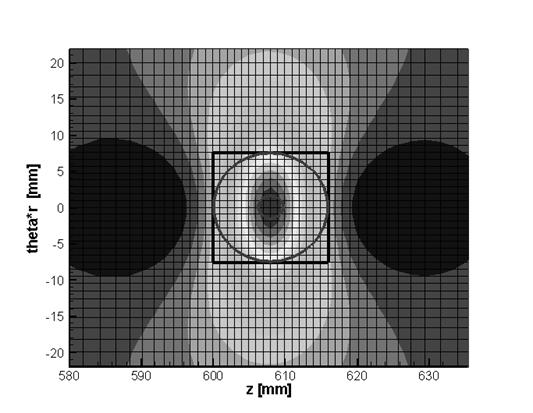
Figure 3. Conical defect: Top and bottom
cone circles are drawn by the dark gray color and white color correspondingly;
uniform grid box is drawn by the black color. The component of EM field inside the
pipe is mapped also.
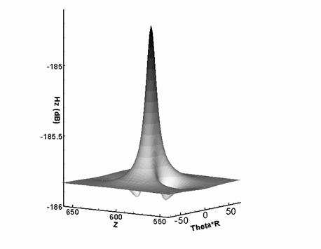
Figure 4. Conical defect: component  of EM field inside the
pipe is mapped of EM field inside the
pipe is mapped
In Figure 4 the same field as in Figure is
presented but as a 3D graph.
In this example we use four
grid levels. The graph of the residual history is shown in Figure 5. We stop
the iterations after 15 MG cycles. Each MG cycle requires about 50
multiplications of the “main” matrix on the finest grid. One can observe that the convergence rate is
sharply drops after 11-th cycle. This is a typical behavior and we can not
still overcome this effect. Note that already 10 MG cycles are enough in this example to obtain the
solution with required accuracy.
Figure 5. Convergence history for 4 grid levels,
the finest grid is 56´80´80
2.2 Modeling of two defects
Here we model the situations
with two “square” defects which are rectangular
parallelepipeds in coordinates (r,θ,z). Both defects have 50% depth
and 16mm side. We consider two cases of location of the defects, the
sequential and the diagonal location, see the scheme in Figure 6. The
coordinate  is shown by the dashed
line. The grid has 60´56´72 cells. is shown by the dashed
line. The grid has 60´56´72 cells.
Figure 6. Two 16mm´16mm defects located in the sequential (left) and diagonal
(right) order. Top view on the pipe wall, 
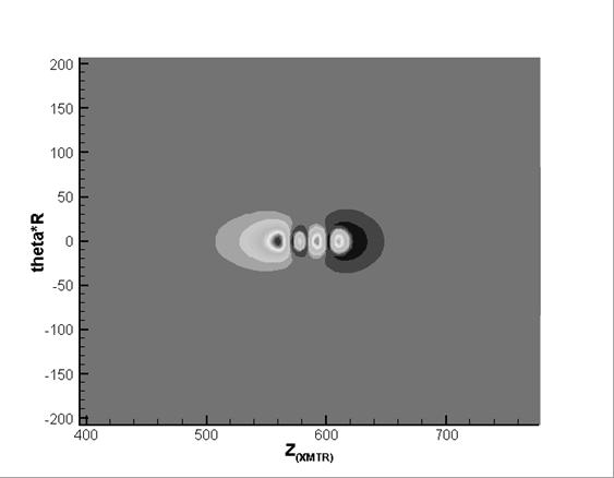 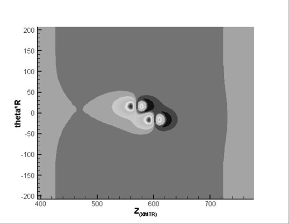
Figure 7. Amplitude of the  -component of the magnetic field; -component of the magnetic field;
sequential (top) and diagonal (bottom) defects
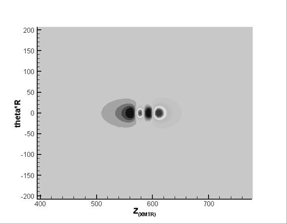 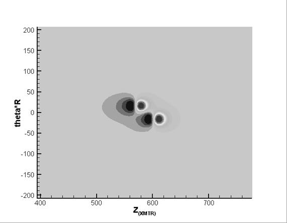
Figure 8. Phase of the -component of the magnetic field;
sequential (top) and diagonal (bottom) defects
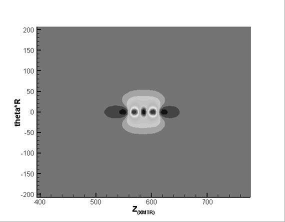 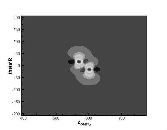
Figure 9. Amplitude of the  -component of the magnetic field; -component of the magnetic field;
sequential (top) and diagonal (bottom) defects
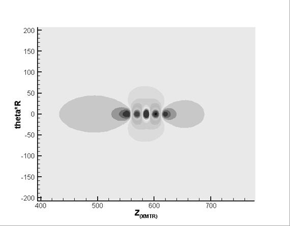 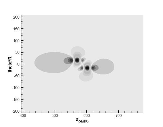
Figure 10. Phase of the -component of the magnetic field;
sequential (top) and diagonal (bottom) defects
Figure 7 – Figure 10 show
amplitude and phase fields of  - and -components of the magnetic field for two cases of
location of the defects mentioned above. - and -components of the magnetic field for two cases of
location of the defects mentioned above.
In our structured
computational grid the smallest cells are located near a defect. Far from
defect the cells are increased in direction of changing of the correspondent
index, i.e. non-uniformly. Therefore there are regions with very thin cells up
to the borders of the computational domain. Superfluous computational points
essentially increase resources which are necessary to solve tasks (memory and
time). But these points do not increase the accuracy of the result. To get over
this issue it is proposed to use a zoom method which consists in the following.
First, instead of solving original
problem

on a sufficiently fine grid,
we consider and solve a problem

on a coarser grid. It is
selected so that global properties of the solution are kept (in particular, on
periphery of a computational domain), but cell-size of this grid is not enough
to accurately describe the solution in vicinity of defects. Then the second problem

is solved for refinement of the solution in vicinity of defects on a fine grid but in smaller domain
 , see sketch in
Figure 11. , see sketch in
Figure 11.
Figure 11. Small 3D computational domain,
cross-section at z=const
Dirichlet boundary conditions
for this problem are taken from the solution of the first problem. The boundary
should be chosen far enough from the defect to be sure that solution of the
first problem is accurate enough there.
It is clear that it is
possible to make next step and solve a problem

having applied the zoom method
to the solution  . However, we restrict us by two steps in this paper. . However, we restrict us by two steps in this paper.
Almost all necessary
information for the solution of a problem using the multigrid method is
organized as an array of pointers to structures. Each structure describes one
multigrid level. It includes geometrical information, environment properties,
arrays of unknown quantities ( ), coefficients of difference equations, right-hand-sides and
some additional information as well as auxiliary arrays. ), coefficients of difference equations, right-hand-sides and
some additional information as well as auxiliary arrays.
In particular, in order to
implement the MG method for discontinuous coefficients we use additional
iterations in the vicinity of coefficients’ contrasts after procedure of
correction prolongation from the coarse grid on the fine one of the previous
MG-level. Technically it is carried out as follows. Regions of coefficients’
contrasts "are covered" by subregions which form 3-dimensional
rectangles in the index space  . For each subdomain . For each subdomain  all interior unknowns all interior unknowns  are additionally
iterated in the smoother, i.e. the corresponding subproblems are additionally
iterated in the smoother, i.e. the corresponding subproblems

are solved more accurately.
The subproblem  is formed by those
difference equations of the main problem which are corresponded to internal
points of the domain. Those unknowns corresponded to an exterior of or its border are not
changed during iterative solution and transferred to the right-hand-side. is formed by those
difference equations of the main problem which are corresponded to internal
points of the domain. Those unknowns corresponded to an exterior of or its border are not
changed during iterative solution and transferred to the right-hand-side.
Data structure of the problem  for the embedded grid
is practically the same as described above. This fact prompts us to use the
same solver for solving of the embedded problem, as for host one. But
recurrence procedure of the MG solver imposes certain limitations on the
structure and use of data. Besides, there are some distinctions in setups of
embedded and host problems. And it is necessary to take into account these
distinctions and to modify procedures of the МG solver to treat both host and embedded problems. for the embedded grid
is practically the same as described above. This fact prompts us to use the
same solver for solving of the embedded problem, as for host one. But
recurrence procedure of the MG solver imposes certain limitations on the
structure and use of data. Besides, there are some distinctions in setups of
embedded and host problems. And it is necessary to take into account these
distinctions and to modify procedures of the МG solver to treat both host and embedded problems.
Note three main distinctions:
1) unlike the host problem which is periodic for the angle  , embedded problem can be both periodic and non-periodic; 2)
borders of the embedded problem should match grid lines of the host problem; 3)
different number and structure of regions along in the embedded and
host problems. , embedded problem can be both periodic and non-periodic; 2)
borders of the embedded problem should match grid lines of the host problem; 3)
different number and structure of regions along in the embedded and
host problems.
We shall give results of two
tests to demonstrate zoom method’s efficiency.
In the first test
the electromagnetic field is calculated for 50% depth outer circular pit having
24 mm diameter. The pipe has internal radius 62.1 mm and 7.7 mm
thickness. The results of two computations are compared. The results of the
first computation are obtained for a maximal possible single-grid problem ( cells). The results of the second computation are obtained
with the help of zoom method when the host problem of cells). The results of the second computation are obtained
with the help of zoom method when the host problem of  cells and embedded
problem of cells and embedded
problem of  cells covering defect
are solved. Both modeling computations have the same grid in the vicinity of
the pit. In Figure
3 the isolines of the absolute value of the function cells covering defect
are solved. Both modeling computations have the same grid in the vicinity of
the pit. In Figure
3 the isolines of the absolute value of the function  are drawn on the plane are drawn on the plane  at radius at radius  . The close neighbor lines correspond to first and
second computations, respectively. . The close neighbor lines correspond to first and
second computations, respectively. 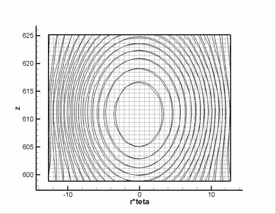
Figure
3. Isolines of the | | at for two calculations: single grid and host + embedded grids. Grid lines are also shown. | at for two calculations: single grid and host + embedded grids. Grid lines are also shown.
Comparison shows a good
coincidence of results. But the volume of the matrix is 8 times less for the
second computation, and CPU time is almost 4 times less (since it was necessary
to solve two problems).
A problem with 87.5% depth
outer circular pit having diameter 6 mm is solved in the second test. The wall
thickness is 8mm (i.e. the remaining wall thickness is 1mm). First the defect
is resolved on the single grid of  cells volume.
Amplitude of the function near the defect at the
section is shown in Figure 4. This is the minimal possible resolution because only
four grid cells put on the pit diameter and rest wall (i.e. solution will be
too inaccurate if we put less than four grid cells on these thin structures). cells volume.
Amplitude of the function near the defect at the
section is shown in Figure 4. This is the minimal possible resolution because only
four grid cells put on the pit diameter and rest wall (i.e. solution will be
too inaccurate if we put less than four grid cells on these thin structures).
It is difficult to estimate
the accuracy of the solution since the resources of PC are not enough to double
resolution of the grid. However, with the help of an embedded grid it became
possible to calculate the defect on a smaller domain for a grid  which has 2 times less
step size in each direction. Solutions obtained on the coarse and fine
(embedded) grids are shown in Figure
5. which has 2 times less
step size in each direction. Solutions obtained on the coarse and fine
(embedded) grids are shown in Figure
5.
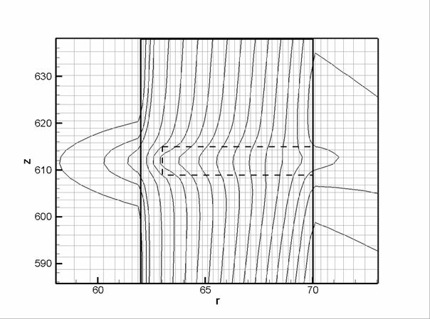
Figure
4. Isolines of || for the single grid solution at the section . Mesh (grey), pipe (vertical solid) and defect (dashed) are
shown as well.
We also present graph of || along z-line at  , see Figure
6. One can observe that both solutions are close to
each other, although finer grid provides a better resolution of course. More
precisely, the relative difference of curves is about 4%. For first and second
derivatives (which model differential sensors) the relative difference achieves
10% to 20%. Believing that the algorithm has the second order of accuracy, we may
conclude that accuracy of the solution on the embedded grid is four times
better, i.e. 1% for function and 3% to 5% derivatives. Note that a good
agreement of both solutions nearby the defects prompts us to use a smaller
domain for the embedded grid, and, therefore, a smaller volume of the latter. , see Figure
6. One can observe that both solutions are close to
each other, although finer grid provides a better resolution of course. More
precisely, the relative difference of curves is about 4%. For first and second
derivatives (which model differential sensors) the relative difference achieves
10% to 20%. Believing that the algorithm has the second order of accuracy, we may
conclude that accuracy of the solution on the embedded grid is four times
better, i.e. 1% for function and 3% to 5% derivatives. Note that a good
agreement of both solutions nearby the defects prompts us to use a smaller
domain for the embedded grid, and, therefore, a smaller volume of the latter.
The problem is model, of
course, but it illustrates possibilities.
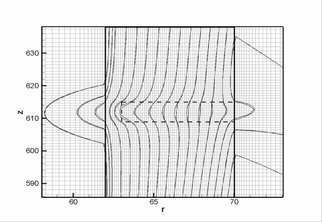
Figure 5. Isolines of || for the single grid solution and embedded grid at the section . Embedded mesh (grey), pipe (vertical solid) and defect
(dashed) are shown as well.
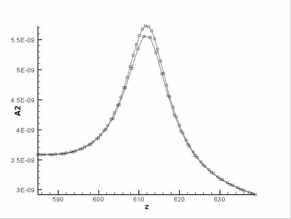
Figure 6. Function || for the single grid solution and
embedded grid at , .
4
Selfconsistent zoom method
In the previous section we
have described the following problem formulation of solution refinement in
zones of large gradients (regions with defects, sources). Let us have the
solution  of electromagnetic
problem of electromagnetic
problem

on a grid  in domain in domain  . Dirichlet boundary conditions for are imposed using
solution of 2D problem in a larger domain . Dirichlet boundary conditions for are imposed using
solution of 2D problem in a larger domain , ,  . .
Then the solution in a
subregion  with defect is refined
by introduction of a finer grid with defect is refined
by introduction of a finer grid  (see Figure 7). The solution (see Figure 7). The solution  satisfies the equation satisfies the equation

with Dirichlet boundary
conditions obtained by restriction of the solution onto the boundary of  . The problem
looks like
, but it can be yet either
periodical or non-periodical with respect to . . The problem
looks like
, but it can be yet either
periodical or non-periodical with respect to .
Figure 7.  -grids near a pit: (gray) and -grids near a pit: (gray) and  (black) (black)
The algorithm is successfully
implemented and it is shown that a more accurate solution can be obtained on
two grids  or it can be obtained
faster than on a single finer grid, see the section above. or it can be obtained
faster than on a single finer grid, see the section above.
Figure 8. Two embedded grids,  -plain section: (fat gray), (thin solid), and -plain section: (fat gray), (thin solid), and  (thin dashed) (thin dashed)
One can consider, in
principle, three and more grids: if, for instance, the casing has two defects
the embedded grids and  could be constructed
independently with possible intersection, see Figure
8. could be constructed
independently with possible intersection, see Figure
8.
Another option with two
embedded grids is the nesting structure:  with finer and finer
grids , . with finer and finer
grids , .
An evident
drawback of the above approach is absence of influence of solution  on solution , what contradicts the elliptical nature of considered
problems. That is why we must take large enough size of in order to diminish
this influence on solution near the defect. on solution , what contradicts the elliptical nature of considered
problems. That is why we must take large enough size of in order to diminish
this influence on solution near the defect.
A more “intelligent” possible
way to reduce the drawback could be consist in organization of the following
iterative process:
§
step #1 is the inconsistent algorithm described above:
we find and and denote  , ,  ; ;
§
step #n (n=2,3,…) solves:
1. The problem

in with a non-zero RHS
defined everywhere inside where the formula

can be calculated;  is an interpolation
operator of is an interpolation
operator of  onto grid points of . onto grid points of .
2. The problem

with the Dirichlet boundary
conditions obtained by restriction operation  of the solution of the solution  onto the boundary of : onto the boundary of :
 . .
If the iterations converge
then one can believe that this the limit solution  is actually the
solution of above an “ideal” problem with the grid adaptive refinement (by
neglecting influence of a small neighborhood of the boundary of domain : one grid level of for both sides of the boundary). is actually the
solution of above an “ideal” problem with the grid adaptive refinement (by
neglecting influence of a small neighborhood of the boundary of domain : one grid level of for both sides of the boundary).
Therefore one can take a
smaller domain comparing the case of
an inconsistent problem.
However our first results did
not give the expected enhance of the algorithm efficiency. Moreover the
iterations diverge sometimes. There are several reasons of the failure, e.g.: a
possible bad construction of the operators and/or (the cubic Cartesian
interpolation); wrong choice of sizes of the embedded domain, etc. We plan to
investigate and overcome the failure in oncoming paper.
References
|