Spacecraft Formation Flying: Relative Orbit Control based on Euler Orbital Elements
|


|
Element |
Definition |
Correlations |
Time Dependence |
|
a > 0 |
|
--- |
--- |
|
|
|
--- |
--- |
|
|
|
|
--- |
|
|
|
|
|
|
|
|
|
|
|
|
|
|
|


The first element a carries an indication of the distance
of the spacecraft from the origin; e
is related to the separation between the two ellipsoids bounding the region of
motion. The third element i is
associated to the maximum height that the spacecraft can reach with respect to
the equatorial plane and to the conservation of the projection of the angular
motion on the same plane. As a result, for i
greater than 90° the orbit is retrograde.
The
shape of the region of motion is fully determined by these three elements. It
shall be emphasized that, due to their definition, a, e and d involve the
computation of x1, x2 and h from the 1st
integrals of motion. To achieve such an outcome expansion till the 4th
order in e (9) and s can be used for
defining a set of mapping relations. The final error gained is of magnitude of
1e-9.
 (9)
(9)
The remnant
elements w0, W0 and M0 map the initial position
of the satellite on the intermediary orbit. They are worked out from the
canonical equations, which involve some elliptic integrals of the 1st
type in the amplitude variables q and y, that respectively
play the role of the true latitude and true anomaly of the satellite on the
intermediary orbit. Once known the initial value of the angular EE, the
osculating terms are computed by first solving for the true anomaly y through equation
(10) and subsequently by using the relations reported in the last column of
Table 1.
 (10)
(10)
4.
Satellite’s Equations for the Perturbed Motion
The
closed form solution of the IM already takes into account the secular effects
due to the first zonal harmonics. As described in Table 1, they affect the last
three EE but they do not modify the shape of the region of motion.
Nevertheless, when dealing with the dynamics in the most general case all the
disturbing contributions of the right side of equations (7) are present. As a
consequence, all the EE would experience some variations with time with respect
to the osculating nominal values of the IM solution. In order to evaluate such
actions an equivalent set of the Gauss’ Variational Equations GVE for the
Keplerian motion can be written by exploiting the variational methodology and
by expressing the disturbances accelerations into a convenient local frame.
Besides,
in order to avoid the numerical issues that arise for circular or polar chief’s orbits, a transformation of the
EE set into a more convenient one, is performed as shown in (11). To the
Eulerian eccentricity value it is summed a vanishing and always positive
quantity. Then the forthcoming semilatus
rectum is employed. For what concerns the Eulerian inclination the same
idea is exploited: from s it is
subtracted a vanishing always positive quantity. The rest of the working set is
constituted by the angular osculating EE.
![]()
![]() (11)
(11)
From now on, this
working set of variables ![]() would be referred as
the state of the system. Though, to
have a straightforward comprehension of the orbit shape, chief’s orbit will be given by a Kepler set. Hence at the initial
instant of time a transformation between that set and the working one is
performed.
would be referred as
the state of the system. Though, to
have a straightforward comprehension of the orbit shape, chief’s orbit will be given by a Kepler set. Hence at the initial
instant of time a transformation between that set and the working one is
performed.
The equations that
express how the state varies due to the action of the disturbances not already
accounted for in the IM problem can be written as follows:
 (12)
(12)


where A
represents the nominal IM solution whereas B
describes how the rest of the accelerations acting on the system affect each
component of the state. Therefore B
is the control influence matrix for
this set of equations and by analyzing its elements it
can be understood when is convenient to correct for each component of the
state, i.e. orbital element. To this extent the set of
Keplerian elements listed in Table 2 is assumed and it is performed a
comparison between the behaviour of each element of B for GVE and equations (12). Trends are evaluated over 2p radians of the true anomaly y; the eccentricity is varied in the range written down in the table.
Tab.2. Keplerian elements set employed for the
evaluation of each term of B
|
a [km] |
e [ad.] |
I [deg] |
W [deg] |
w [deg] |
M [deg] |
|
7550 |
[0.001,0.3] |
48 |
0 |
10 |
[0,360) |
Figure 1 and 2 illustrate the plots obtained, dashed lines refer to the
minimum value of eccentricity here considered. In some subplots it is useful to
mark, by a square on the axis of abscises, the moment when the true latitude q is ± 90°; respectively the north and south poles of
the positive orbits. Every picture is called according to the position of the
element that represents into the control influence matrix. Unit dimensions are
coherent according to such dimensional equations.
For what concerns the Keplerian motion, i.e. Figure 1, it can be noted that
B11 and B21 vary proportionally to sin(y); B12 oscillates around a mean
positive value depending on 1/r(y); in B51, B52,
B61, B62 small values of eccentricity amplify the nominal cos(y)
trend. Such an eccentricity effect can be appreciated also in B22, B33, B43,
B52, B53 and B62
where r(y) multiplies
the oscillating factor. Finally B33
is proportional to cos(q) whereas B43 and B53
vary with r(y)sin(q). As
each colon of B introduces the action
of an acceleration into one of the local-frame directions, it is easily derived
that in order to correct on semi-axes, eccentricity and mean anomaly in-plane
manoeuvres must be used. Changes in inclination and longitude of ascending node
are performed by out-of-plane actions, more efficiently respectively at the
Equator and at poles. The perigee anomaly can be affected by all the
accelerations. Further information is carried by the order of magnitude of each
component of B.
Figure 2 reports the control influences components for the Euler problem.
Due to the intrinsically more complex problem carried out and to the different
choice of state variables, the subplots present different behaviours with
respect of the previous ones. In particular the second and third equations now
regard p and s and on them accelerations in every direction can produce effects.
Together with the strengthening due to small eccentricity values already
pointed out before, here there are amplifications due to the dependence of the semilatus rectum on e. This effect is clearly visible in B23, B33,
B43, B53. As a consequence, in order to correct produce
changes on p and s accelerations either in-plane either out-of-plane can be
provided. Still the order of magnitude completes the information required.
Fig.1. Kepler
problem: control influence matrix B
on one orbit. The dashed trends refer to e
= 0.001.
Fig.2. Euler
problem: control influence matrix B
on one orbit. The dashed trends refer to e
= 0.001.
5.
Relative Orbit Control Scheme
Satellites’
relative motion can be fruitfully described through differences in the orbital
elements associated to the chief and
the deputy spacecrafts. Generally
this methodology gives a straight physical insight of the shape of the relative
trajectory and a relative orbit control
scheme can be established on such an approach. To this extent, if EE are
employed, equations (12) need to be used to compute how the state ![]() varies when control
and disturbance accelerations act on the deputy satellite. The reference
relative orbit is defined starting from the chief’s
EE. As relative control is sought, no further perturbing actions work on the
reference spacecraft:
varies when control
and disturbance accelerations act on the deputy satellite. The reference
relative orbit is defined starting from the chief’s
EE. As relative control is sought, no further perturbing actions work on the
reference spacecraft:
 (13)
(13)
The controller receives as input the error with respect to the reference
state and elaborates which accelerations to provide in order to contrast it:
 (14)
(14)
To avoid to insert
at every time step errors connected to the mappings between EE and ![]() (11), proper initial
conditions are given to the reference state, i.e. dashed block in Figure 3, and
(11), proper initial
conditions are given to the reference state, i.e. dashed block in Figure 3, and
![]() is also propagated.
Due to the fact that an intermediary orbit is assumed as the reference to be
tracked, the controller counteracts only the remnant disturbances and errors in
the initial conditions.
is also propagated.
Due to the fact that an intermediary orbit is assumed as the reference to be
tracked, the controller counteracts only the remnant disturbances and errors in
the initial conditions.
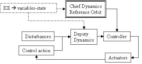
Fig.3. Control scheme structure: feed-back based on
information in terms of EE.
The disturbance
actions considered in this study are the remnant zonal harmonics of the Earth
gravitational field, till the 6th order. In the actuation block it
is taken into account the maximum acceleration provided by the engines, here
assumed as 0.01 m/s2.
6. Design of the Controller
According to (14) the dynamics of the error is given by:
![]() (15)
(15)
By defining V as a positive defined function of de and by taking its time
derivatives on the system’s trajectories, u and the matrix P can be designed in order to have an asymptotic
stable closed-loop error dynamics, according to:
 (16)
(16)
The real
accelerations the controller shall provided are computed as follows:
 (17)
(17)
hence the pseudo-inverse
of the 6x3 matrix B is involved. The
control is composed by a part proportional to the tracking error, one that
compensates the disturbances and one that accounts for the discrepancies
between dynamics of the reference and the deputy.
The first one is the responsible for recovering the initial error and gains,
i.e. terms of the diagonal positive defined matrix P, shall be properly tuned. The second term cancels the effects of
the disturbances, hence turns out in an oscillating contribution still present
after that the intermediary reference orbit is established. The last component,
due to the FF description in terms of orbital elements, is small: differential
elements of order 1e-3 can give rise to a large formation geometry.
If ![]() were the identity matrix, then P could be simply chosen from the time duration of the transient
for recovering the initial error. However, both
were the identity matrix, then P could be simply chosen from the time duration of the transient
for recovering the initial error. However, both ![]() involves some numerical issues
and
involves some numerical issues
and ![]() carries with itself the natural
couplings intrinsic in the nature of the phenomenon. Figure 4 and 5,
respectively depict the element-by-element trends over 2p radians of those
two matrixes. The first picture deals with the eccentricity’s span of Table 2,
whereas the weighting matrix is computed only for e = 0.05. The pseudo-inverse presents some picks when the
determinant of the quantity
carries with itself the natural
couplings intrinsic in the nature of the phenomenon. Figure 4 and 5,
respectively depict the element-by-element trends over 2p radians of those
two matrixes. The first picture deals with the eccentricity’s span of Table 2,
whereas the weighting matrix is computed only for e = 0.05. The pseudo-inverse presents some picks when the
determinant of the quantity ![]() decreases to quite zero, and
especially for small eccentricity values. As a consequence the real control
commands turn out to be amplified and edgier than the ideal ones. Figure 5
allows to evaluate the coupling effects among the control actions. In order to
accomplish it the diagonal terms should be monitored: they should be dominant
with respect to the extra-diagonal ones, to be likely the ideal situation
represented by the identity matrix. The first two rows, and columns due to
symmetry, satisfy this requirement. All the angular terms, on the contrary, do
not fulfil it. And, even whenever for almost the whole orbit the diagonal term
is greater than the correspondent extra-diagonal ones, they all are of the same
order of magnitude anyway. To fully understand this behaviour it is useful to
go back to Figure 2. There, each column can be viewed as how the correspondent
control component acts, at a fixed true anomaly, on every element of the state.
For what concerns the radial and transversal accelerations, respectively first
and second columns, it can be noted that the most dangerous couplings arise
between pericentre and mean anomaly and between s and p. In this second
case, however, the order of magnitude of the different possible control actions
fixes what is more convenient, hence compensates the before mentioned coupling.
The out-of-plane action generates a dangerous combined effect between
pericentre anomaly and longitude of ascending node. Actions on s and W are naturally
decoupled.
decreases to quite zero, and
especially for small eccentricity values. As a consequence the real control
commands turn out to be amplified and edgier than the ideal ones. Figure 5
allows to evaluate the coupling effects among the control actions. In order to
accomplish it the diagonal terms should be monitored: they should be dominant
with respect to the extra-diagonal ones, to be likely the ideal situation
represented by the identity matrix. The first two rows, and columns due to
symmetry, satisfy this requirement. All the angular terms, on the contrary, do
not fulfil it. And, even whenever for almost the whole orbit the diagonal term
is greater than the correspondent extra-diagonal ones, they all are of the same
order of magnitude anyway. To fully understand this behaviour it is useful to
go back to Figure 2. There, each column can be viewed as how the correspondent
control component acts, at a fixed true anomaly, on every element of the state.
For what concerns the radial and transversal accelerations, respectively first
and second columns, it can be noted that the most dangerous couplings arise
between pericentre and mean anomaly and between s and p. In this second
case, however, the order of magnitude of the different possible control actions
fixes what is more convenient, hence compensates the before mentioned coupling.
The out-of-plane action generates a dangerous combined effect between
pericentre anomaly and longitude of ascending node. Actions on s and W are naturally
decoupled.
Taking
into account all these considerations the structure of the gain matrix P can be employed to limit some of those
issues. In [4], where an approach on orbital elements was also exploited, it
was suggested how a time varying gain matrix turns out to be useful to help in
supporting the natural dynamics of the system instead of fighting it. Together
with such a heritage, here it is pursued the idea of creating some differences
in the order of magnitude among some of the tracking error contributions to
unbalance the equilibrium in the structure of
![]() that would lead to a steady-state
error.
that would lead to a steady-state
error.
Tab.3. Variable gains: structure and values assumed
for the incoming simulations.
|
Structure |
P constant |
Amplitude |
Speed N |
|
|
0.005 |
--- |
--- |
|
|
0.005 |
--- |
--- |
|
|
0.000005 |
0.005 |
2 |
|
|
0.000005 |
0.005 |
2 |
|
|
0.000005 |
0.0001 |
2 |
|
|
0.000001 |
0.00001 |
2 |
In Table 3 the final choice of structure and numerical values of the
gains is resumed. The first two gains are constant as their correspondent equations
are decoupled. They are mainly corrected by the in-plane accelerations and the
magnitude of the gain was derived by trading off the time for recovering the
initial error and the maximum acceleration that the engines can provide. All
the other gains are composed by a constant term plus one varying along the
orbit. The idea of the constant contribution is to switch off some “noise”
information when it is not needed. On the contrary, when the satellites reaches
convenient positions corrections on same components of the state are encouraged
by the time varying part. Then the amplitude gives the magnitude effect whereas
the exponent, i.e. velocity, gives how fast the switching is activated. For
what regards s and W, it is
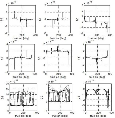
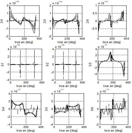
Fig.4. Euler problem: pseudo-inverse on one orbit.
The dashed trends refer to e = 0.001.
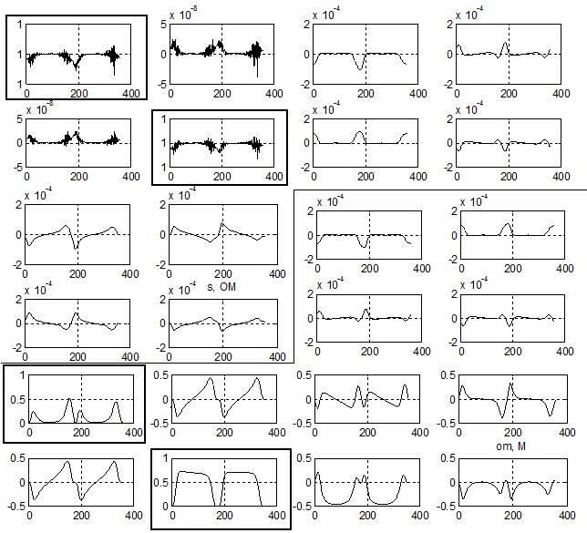
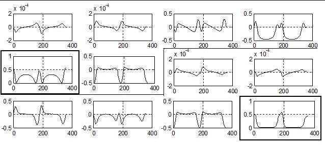
Fig.5. Euler problem: matrix that weights the
control commands evaluated on one orbit for e = 0.05. True anomaly is on the
abscisses, whereas state-component weights are on the ordinates. Sectors divide
the rows; diagonal terms are highlighted.
simply encouraged the natural tendency of correcting
them respectively at Equator and poles. Their amplitude is the same. Regarding
the last two equations, again it is exploited some complementary scheduling of
the corrections. Nevertheless, due to the structure of B, when acting on one also the other is affected. The only option
available is to emphasized some difference in order of magnitude, together with
the one performed when the command is switched off by the angle dependency. For
all the time varying quantities, the action is not too impulsive: a smooth
behaviour is preferred.
7. Simulations and Results
In the simulations here presented, as a benchmark, it is considered the
establishment of a relative motion with respect to a chief satellite on an eccentric orbit, as performed in [4]. Usually
the eccentricity of the reference satellite involves some issues in modelling
and controlling the relative dynamics. All the Keplerian initial elements of
the chief’s orbit are reported in
Table 4. They are provided in order to give a straighter insight of the
problem. According to the control scheme depicted in Figure 3, this information
is first translated into the correspondent Eulerian set and subsequently in the
working one.
Tab.4. Chief initial conditions: Keplerian orbital
elements.
|
a [km] |
e [ad] |
i [deg] |
W [deg] |
w [deg] |
M [deg] |
|
7550 |
0.05 |
48 |
0 |
10 |
80 |
The reference orbit is defined from the chief EE set through a difference in
orbital elements. Generally the approach of defining the relative motion
through differences between such constants of the two satellites is convenient
for at least the following reasons. First there is no need to solve the
equations of relative motion to derive information about the spacecraft
position, as for the dynamics expressed in a local frame. Secondly it doesn’t
rely on any hypothesis embedded in the modelling scheme, such as small relative
radii for linearization purposes or small eccentricity values of the reference
orbit like for Hill-modelling extensions. In the introduction paragraph it was
pointed out how the choice of the target relative motion is a crucial aspect
for real FF missions. Coherently, when possible, invariant orbits are sought as
they do not require strong and expensive control for position maintenance
during their lifetime. By exploiting Eulerian orbital elements it is possible
to define relative motions which are insensitive up to the effects caused by
the presence of J3. Such orbits arise from the observation that, for
the nominal IM, the elements connected to the shape of the region of motion do
not vary with time. Moreover all the coefficients related to the time
dependences in the remnant elements are function of exactly those
shape-describing elements. Hence, in order to have a frozen-bounded relative orbit, taking into consideration the
deformations due to the first zonal harmonics of the gravity potential, it is
simply necessary to ask that all the satellites have matching deviations from
the nominal behaviour, i.e. same time derivates of Eulerian longitude of
ascending node, pericentre anomaly and mean anomaly. Nevertheless, by asking
this for all the angular elements simultaneously turns out into a poor freedom
in designing the shape of the relative motion. In this case, in fact, only
extensions of Leader-Follower configuration, or oscillations in the out of
plane direction are achievable together with a displacement into the along-track
direction fixed by a difference in mean anomaly. However, if it can be accepted
to perform some corrections on the relative orbit, one of those three
constraints can be relaxed, hence establishing some circular motion of the deputy satellite with respect to the
reference one. It shall be emphasized that, as here EE are employed, the before
mentioned further corrections are tiny because they have only to compensate for
the disturbances not already accounted for in the IM.
The relative orbit used in the simulations is
defined in Table 5 and it is a J2-J3 invariant relative
orbit of the type of a General Circular Orbit GCO. The designing parameter
assigned consists in a difference in the Eulerian inclination; differences in a and e are consequently derived to meet the constraints of matching time
variations in true latitude and longitude of ascending node between the two
satellites.
Tab.5. Definition of the relative orbit to be
tracked, through differences of EE.
|
da [m] |
de [ad] |
di [deg] |
dW [deg] |
w [deg] |
M [deg] |
|
-0.652 |
0.577e-3 |
0.006 |
0 |
0 |
0 |
Simulation depicted in Figure 6 refers to the establishment of the
target orbit given in Table 5, when the deputy initial error is given in terms
of differences in EE as follows:
![]() (18)
(18)
On the secondary satellite
disturbances are acting as well. In the subplots are respectively shown the
transients of the tracking errors in a
and p, in the left-top corner, of s and of all the remnant angular orbital
elements. In the last view it is sketched the trajectory the deputy performs while trying to achieve
the target orbit, plotted in the Hill frame centred in the chief satellite. As expected from the structure of the control
weight matrix, a and p present an ideal-like behaviour, and
quickly recover their initial errors. Also s
slowly moves to the requested value. The other angular elements, on the
contrary, present a transient phase and then stabilize on a steady-state value
different from the required one, i.e. zero. Such a behaviour was predicted when
analyzing the couplings among such terms, and, in the Hill frame, it turns out
into a relative orbit of the proper shape but displaced from the target one of
a quantity composed by the combination of the steady-state errors on pericentre
and mean anomaly. Except for the variables shown in the first subplot, for whom
gains were set to be constant, it can be easily recognizable how corrections
are performed with an impulse-like approach, coherently with the exploitation
of the dynamics of the system. The total DV imparted for performing this
reconfiguration is 15.73 m/s, see Table 6, hence greater than what reported in
[4] for a similar manoeuvre. However, it shall be remarked that, such a
performance index depends on the gains’ design, the consequent thrust profile,
the type of relative orbit sought and, finally, the initial mean anomaly value.
Some optimization of the control features shall be accomplished focused on each
specific application. For what concerns the final goal, however, a finer result
is here achieved as osculating elements are used instead of mean ones, and
target orbit already takes into account also the J3 effect.
Fig.6. 1st simulation: Lyapunov-like
control. Initial condition and gains are summarized respectively in Tables 4, 5
and 3. Initial errors are given by (18).
In order to avoid
the steady-state error, the action of the controller can be enriched by adding
a contribution proportional to the error with respect to the aimed value of the
pericentre anomaly as follows:
![]() (19)
(19)
The idea is to
force some further action on the system, hence spending something more, to
impose some artificial ranking on the corrective manoeuvres to be performed.
The gain of this extra contribution is fixed trading off the time needed for
recovering that component of the tracking error, the maximum acceleration
provided by the engines and the subsequent increase of DV required. According to the
dynamics, the proportional part (19) shall be introduced in (16) in order to
compute the real commands that the actuators shall provide:
 (20)
(20)
The matrix BP is a design parameter and
it regulates which control acceleration, i.e. direction, to use to impart such
a further action. Finally, the contribution is reinserted in the equation
through the control influence matrix B
computed at the current state of the deputy.
In Figure 7 there are presented the results gained by a simulation in which the
new control action is employed. All the rest of the environment is kept as
before. What immediately catches one’s attention is the different behaviour of
the tracking error of s and of the pericentre anomaly, of course.
Fig.7. 2nd simulation: Lyapunov-like
control and proportional part on the error in PA. Initial condition and gains
are summarized respectively in Tables 4, 5 and 3. Initial errors are given by
(18).
Now
the out-of-plane action is more effective and the inclination of the deputy’s orbit changes more, till the
last orbit insertion in the target’s plane is accomplished. Because of the
artificial ranking imposed on the corrections, the tracking errors on every
component of the state, with the exception of the mean anomaly go to the
expected value. Yet the steady-state error is decoupled, hence according to the
physics of the problem this means that, by simply accomplishing the same
manoeuvre some time, i.e. final mean anomaly error, before or later, the
expected target trajectory is established.
Fig.8. 3rd simulation: all the features
employed in the 2nd simulation are kept. However here a correction
in the initial time of the manoeuvre is performed.
Fig.
9. Control accelerations’ profiles needed for
the 3rd simulation. They are expressed in the [S, T, B] local frame.
Fig.10. 4th
simulation: Lyapunov-like control and proportional part on the error in PA
given by only the radial component S. Initial condition and gains are
summarized respectively in tables 4, 5 and 3. Initial errors are given by (18).
A proper correction of the initial time of the manoeuvre is performed.
Fig.11. Control accelerations’ profiles needed for
the 4th simulation. They are expressed in the [S, T, B] local frame.
Figure 8 presents
the result gained when, together with the complete control law, correction in
difference of Eulerian mean anomaly on the definition of the target relative
orbit is set. Both the amount of the correction and of the final errors gained
are reported in Table 6. Figure 9 shows the control accelerations that the
actuators shall provide. Due to the further action the DV required increases with
respect to the first simulation performed. Despite this, the final result is much
more accurate.
So far the action
of the proportional part was carried out by all the three components of the
control acceleration, and all of them play a role according to Bd. Nevertheless by
considering that the proportional contribution was added to compensate the
error in pericentre anomaly, which, according to the dynamics of the system is
primarily affected by the in plane corrections, it is convenient to demand all
that work to the component S of this supplementary control. The other two
components B and T would only insert respectively, a strong disturbing coupling
action with the out of plane dynamic and a fighting strategy with respect to
the approach fixed for the gains, see Table 3. To achieve this, it can be used
the matrix BP which
compares in (20). Figure 10 presents the result gained when the correction
proportional to the error in pericentre anomaly is performed by the
radial-in-plane component S. The
profile of s reveals how the
manoeuvre less involves changes in inclinations, with great benefits on the
total DV spent, see Table
6. Figure 11 shows the correspondent control accelerations, hence it is
possible to compare the different behaviour of B in the two cases: now it only works for part of the control law.
Finally, as a result, the real trajectory covered by the deputy presents a very different profile, coherently with the fact
that small changes in the orbital elements reflect into great modifications of
the relative dynamics of the spacecrafts, according to the way they are
defined.
Tab.6. Final errors gained in terms of EE and
correspondent DV spent by the control action performed in the
different simulations presented before.
|
Final Error |
1st simulation |
2nd simulation |
3rd simulation |
4th simulation |
|
da [m] |
1.8569e-3 |
3.9621e-3 |
2.3456e-4 |
5.68e-5 |
|
de [ad] |
2.11e-9 |
4.99e-9 |
6.67e-11 |
8.6e-11 |
|
di [deg] |
1.5744e-5 |
3.7236e-5 |
4.741e-7 |
7.1e-7 |
|
dW [deg] |
6.4072e-4 |
1.8310e-4 |
6.489e-6 |
2.24e-8 |
|
dw [deg] |
0.051935 |
1.3299e-4 |
4.701e-6 |
2.572e-7 |
|
dM [deg] |
0.125814 |
0.068952 |
0.000312 |
0.000204 |
|
DV [m/s] |
15.73 |
24.29 |
24.13 |
20.79 |
Final Remarks
In this work a
relative orbit control scheme for formation flying missions is addressed. The
study relies on the exploitation of orbital elements, as they provide a clear
physical insight in the description of the dynamics of a point with respect to
a massive body. By supporting this approach, relative target orbits and
relative motion are expressed respectively by differences in Euler orbital
elements and in their variations in time. Eulerian orbital elements represent a
convenient mathematical tool as they already involve all the most effective
phenomena that occur in the formation flight of small satellites in low energy
orbits. However, the intrinsic complexity of the problem moves from the modelling
level to the design of the controller: the equations that rule the time
variation of the Eulerian elements for the perturbed motion are highly
nonlinear and intrinsically coupled.
The proposed
control law is based on the theory of Lyapunov. Besides gains that vary across
the orbit are used. In order to avoid a final steady-state error a further
control action is introduced: it consists in a contribution proportional to the
error in pericentre anomaly. Due to such a complex design process, for each special
application it is suggested to accomplish an optimization study to work out
what are the best gains’ values and starting time of the reconfiguration
manoeuvre, taking into account the available thrusters. This means that, the
great enlargement of possibilities that such a comprehensive modelling tool
offers, both in terms of accuracy and generality of the situations that can be
described, is paid by a certain lack of robustness which affects the control
scheme. From a higher level point of view, the exploitation of such a rich
modelling tool, together with the proposed control scheme, requires a parallel
investigation of the management of the
operations during the whole formation flying mission: scheduling of different
working modes.
Despite of these features,
the proposed approach can be employed either for performing reconfigurations of
the formation, either for accomplishing fine control phases, i.e. during
scientific segments. The first chance is based on the idea of exploiting the
natural dynamics of the phenomenon to achieve expensive manoeuvres; the second
one gets benefits from the fact that Eulerian elements already take into
account zonal effects till J3 and partially J4. For what
concerns tight formations, it is suggested to carry out also a check for
collision avoidance: as mentioned when analysing the results gained, small
changes in the orbital elements can reflect into great modifications of the
relative motion.
Finally, beneath
this work an introduction on the design of convenient relative orbits is
presented. The idea is to match the time variations of some orbital elements,
caused by the environment, in the definition of the orbit to be tracked. As a
result the control has to balance only the further disturbances not already
taken into account in the model. The simulations run deal with the
establishment or reconfiguration of a formation into such frozen-bounded
motion.
References
1. W. H. Clohessy and
R. S. Wiltshire, “Terminal Guidance
Systems for Satellite Rendezvous”, Journal of the Aerospace Sciences, pp.
653-658, Sept. 1960.
2. S. S, Vaddi, “Modelling and Control of Satellite Formations”, Ph.D. thesis c/o
Texas A&M University, May 2003.
3. H. Schaub and K. T. Alfriend, “J2 Invariant Relative Orbits for Formation
Flying", International Journal of Celestial Mechanics and Dynamical
Astronomy, Vol. 79, 2001, pp. 77-95.
4. H. Schaub, S. R.
Vadali, J. L. Junkins and K. T. Alfriend,
“Spacecraft Formation Flying Control using Mean Orbit Elements”, Journal of
the Astronautical Sciences Vol. 48, No. 1, Jan.–March, 2000, pp. 69–87.
5. S. R. Vadali, H. Schaub and K. T. Alfriend, “Initial Conditions and Fuel Optimal Control
for Formation Flying of Satellites”, AIAA Guidance, Navigation, and Control
Conf., July–Aug. 1999.
6. S. S. Vaddi, K. T. Alfriend, S. R. Vadali
and P. Sengupta, “Formation Establishment and Reconfiguration Using
Impulsive Control”, Journal of Guidance, Control, and Dynamics Vol.28. No.
2, March-April 2005, pp. 262.
7. J.D. Biggs, V.M. Becerra, S.J. Nasuto, V.F.
Ruiz and W. Holderbaum, “A Search for
Invariant Relative Satellite Motion”, ARIADNA Study 04/4104.
8. M. Sabatini, D. Izzo and G. Palmerini, “Analysis and control of convenient orbital
configuration for formation flying missions”, 16th AAS/AIAA Space Flight
Mechanics Conference, Tampa, Florida January 22-26, 2006.
9. E. P. Aksenov, “Theory of the Motion of Artificial Satellites of the Earth”, ed. Nauka,
Moscow, 1977 (in Russian).
10. V. G. Demin, “Motion of an artificial satellite into a noncentral gravitational
field”, ed. Nauka, Moscow, 1968 (in Russian).
11. E. P. Aksenov, E. A. Grebenikov and V. G.
Demin, ”Generalized Problem of the Two
Fixed Centres and its application in the theory of motion of artificial
satellites of the Earth”, Russian Astronomical Journal, Vol.40, No.2,
pp.363, 1963.